Here is the link:
http://members.cox.net/fbirchmore/cse%20190a/blog%202-26-06/2-26-06.html
Sunday, February 26, 2006
Monday, February 20, 2006
Detecting the Letter 'e': success!
To see my progress, click the provided link. I've grown tired of trying to fit everything into these little narrow blog spaces. After fumbling around with images, I activated my ISP web space.
http://members.cox.net/fbirchmore/cse%20190a/blog%202-20-06/2-20-06a.html
http://members.cox.net/fbirchmore/cse%20190a/blog%202-20-06/2-20-06a.html
Sunday, February 12, 2006
Weak Classifiers for the Letter 'e': success!
Well, I finally generated some weak classifiers that yield distinct curves with fairly good separation.
Calculating the Error Rate
Using the filters that I had previously generated, I calculated the error rate experimentally. To do this, I removed the first 10 positive examples from the positive training set. In other words, I removed 10 images of the letter 'e' from the pool of images that I used to generate the filter response curves. These 10 images made up my testing set. For each filter, I then calculated its response to all of the positive training images ( excluding the 10 images that I had removed for a testing set ) and its response to all of the negative training images. In order to fit gaussian approximations to these responses, I calculated the mean and standard deviations of each group of responses --calculating for the positive and negative responses separately.
To calculate the actual error rate, I performed the following algorithm:
for each filter:
begin
0) initialize an integer value to 0 for the current filter. This value will accumulate "votes"
based on the classification of the test images.
for each image in the testing set: ( ie: the set of 10 positive images set aside )
begin
1) convolve the current filter with the current image to yield a response --call it x
2) using the calculated means and standard deviations for this filter, (call them pm, ps,nm, ns for positive mean, positive standard deviation, negative mean, and negative standard deviation) retrieve likelyhood estimates for x. Call them P(x | p) and P(x | n) for positive and negative likelyhoods, respectively. Since the estimated gaussians represent PDFs (Probability Density Functions), P(x | p) and P(x | n) are calculated as follows:
P(x | p) =(1/(sqrt(2*pi)*ps)) * exp(-((x-pm).^2)/(2*ps^2));
P(x | p) =(1/(sqrt(2*pi)*ns)) * exp(-((x-nm).^2)/(2*ns^2));
3) plug each likelyhood into Bayes' equation to get the probability of being an 'e' and not being an 'e'. Call them P(p | x) and P(n | x), respectively. Let P(p) and P(n) be the prior probabilities for 'e' and not 'e', respectively. Remember that P(p) and P(n) represent the probability of a random letter on a sheet of paper being an 'e' and not being an 'e'.
P(p | x) = P(x | p) * P(p)
P(n | x) = P(x | n) * P(n)
Note that in Bayes' equation, these terms are usually divided by the probability of a feature vector occuring. Since there are only two different possibilities for classification, 'e' or not 'e', the probability of a feature vector occuring is ignored since these probabilities will just be compared to each other, as you will see below.
4) classify the current test image by comparing the probabilities computed in step 3:
if P(p | x) > P(n | x), then the image is classified as 'e', so output 1
if P(n | x) > P(p | x), then the image is classified as not 'e', so output = 0
This essentially means that if an image has a greater probability of being an 'e' than not being an 'e', then it should be classified as an 'e' (and vice-versa). This reminds me graphically of an individual step in K-Means in that at any individual step in computing a boundary for K-Means, K-Means simply classifies an input value as being whichever mean that value is closest to in euclidean distance.In contrast, the type of Bayes' classifier that I have implemented classifies an input value as one class or another based on how many standard deviations away from the mean of each curve it is.
5) for the current filter, add the following to the running total of votes for the current filter:
1 - if the input image is an 'e' and it was classified as such
0 - if the input image is an 'e' but it was classified as not an 'e'
Since the test images are known to be positive (ie: known to be 'e' ), the result of the classifier can simply be added to the current vote tally for the current filter.
end
end
After these steps were run, each filter was left with a number of votes correponding to the number of 'e's classified correctly. If a filter has a vote tally of 10, for instance, this means the classifier built from this filter classified all 10 of the test images correctly as 'e'. Since the testing images are known to be 'e's ahead of time, they are referred to as labelled.
Results
Best Filter
I ran the aformentioned algorithm for all filters and for 10 positive test images. I then arranged the filter numbers according to how many votes each one had. Here is an example of one of the best filters, showing histograms of its training set with fitted gaussians (first below) and the same filter with just its gaussians displayed (second below)
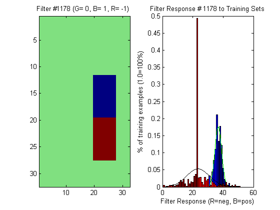

In my most recent blog posting, I displayed a filter and its response as two nested gaussians. From the experiments I have performed since then, I realize that this graph from the previous posting was obviously incorrect. When displaying the gaussians, the prior probabilities should not be taken into account. The gaussians alone are only used to compute a likelyhood estimate --not a probability. The introduction of scaling by the prior probabilities should only be added when classifying --not visualizing the PDF. I also discovered a minor bug that was causing the mean values to be shifted incorrectly. These problems have been fixed since then.
Initially, I thought that my intuition about the location of possible features did not directly translate to the use of filters in Bayes' classifiers. Now, I can see that my intuition is confirmed by the location of this filter at almost the same location as the nested gaussian in the previous post.
Worst Filter
Here is an example of one of the worst filters, displayed in the same manner as the previous two images:
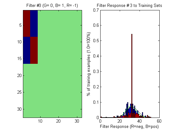

Here, the gaussians almost match up meaning that the classification of an input image is almost entirely dependent on the prior probabilities. This means that if this filter were to be used to build a classifier, then training sets might as well not have been collected at all.
Global Analysis of Filter Performance
The graph below shows y percentage of filters that classified x percentage of test images correctly:

If you observe the far left-hand column, you can see that 80% of the filters are completely worthless in that they were not able to identify any letter 'e's correctly out of the 10 test images. One of the main advantages of Adaboost is that the presence of these useless filters will not affect the resulting strong classifier --Adaboost will automatically throw these filters out and choose the best ones. If you look at the far right-hand column, you will see that fewer than 5% of the filters classified all 10 of the test images correctly. It could be that the 10 test images I chose have attributes that make them easy to recognize by the top 5% of classifiers. Perhaps the top 5% classifiers would fail miserably with negative examples or most other positive examples. Adaboost will help to avoid this scenario by forcing the classifiers to focus on the most difficult examples.
The following graph represents the percentage of test images classified correctly for each filter number. For reference, an image of the filters is shown below it:
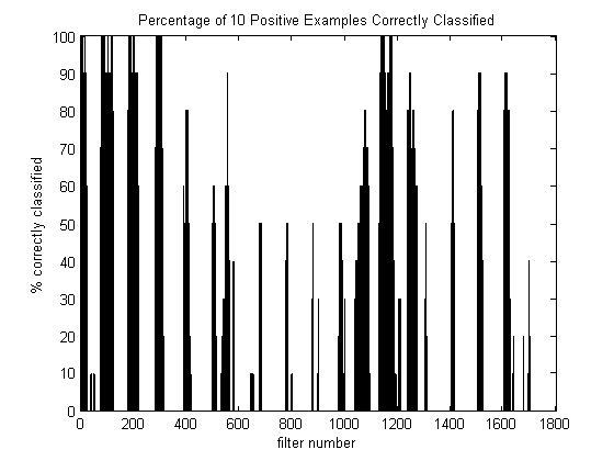
From the graph, there are many instances where a small group of filters perform exceptionally well while a different group in close proximity performs poorly. Though only 10 examples were used to test, the advantage of generating many different filters is apparent. If intuition alone is relied upon for the construction of a filter, then it could be missing an area of interest by a few pixels that might make the difference between achieving good classifications or not. Regardless of how good human intuition is, it is handy to rely upon the precision of a computer to pick up the slack.
What's Next
The next step will be to implement Adaboost using the weak classifiers I have constructed. I may need to generate more filters, but I will keep the number small for now for the sake of computation time.
Training Footage of Soda Cans
I obtained training footage from Robart III of soda cans! I will post on this once I clean up the raw footage a bit.
Saturday, February 04, 2006
Detecting the letter 'e'
Last week, I was reading over Dlagnekovs code in an attempt to understand how he used Adaboost. Dlagnekov's code is very clean and easy to understand. However, I had a difficult time discerning details from the code, such as how his Bayes classifiers work. I was also unclear as to how one is able to use a training set of images in conjunction with a group of weak classifiers to generate ROC curves. It is one thing to read theory on this subject, but I needed to see a concrete example.
I wrote up a trivial example of generating a training set and applying classifiers on paper, but I wasn't getting a nice looking graph with two distinct humps. Instead, I was getting an almost flat curve for the positive training set and two impulses for the negative training set. I talked with my professor and he said that the type of classifiers Dlagnekov uses are statistical classifiers, meaning that in order to get good curves, one must have a large number of positive and negative classifiers. He suggested that I implement an Adaboost method for detecting the letter "e" (lowercase) on a white sheet of paper before attempting to detect soda cans. He provided me with a link to a research paper that was first printed out with a dot-matrix printer, then scanned in and converted to PDF format. This means that the letters in the paper vary quite a bit, making the detection process nontrivial. He suggested that I use this paper to generate positive and negative training examples as well as using it to test my implementation. Here is a link to the paper I used:
http://www-cse.ucsd.edu/classes/sp02/cse252/foerstner/foerstner.pdf
Creating the Positive Training Set
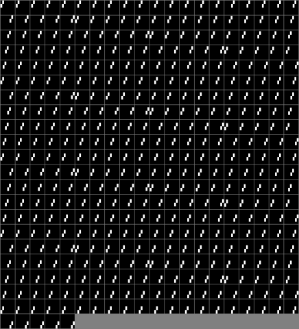
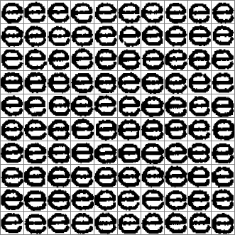
I wanted each image to be 32x32 pixels so I zoomed in with Adobe Reader to a 400% scale and took a screenshot. I then pasted the screenshot into Windows Paintbrush and manually cut out every lowercase "e" in the image. I repeated this process until I had 100 different lowercase "e"s in a single bitmap image. This image was then run through a Matlab script I wrote where, when I click the center of each letter 'e', a 32x32 pixel region surrounding the selected location is automatically exported as a new bitmap file. I also saved the image with every lowercase "e" removed so I could later use this e-less image to create negative training examples. Since the research paper was scanned-in with a dot-matrix printer, the quality of each letter e is slightly different --some e's are almost perfect while others look more like o's. These images make up my positive training set, meaning they are examples of what the letter 'e' should look like. Here is a composite image consisting of all of the 32x32 images of the letter 'e' created for visualization purposes using a matlab script:

Creating the Negative Training Set
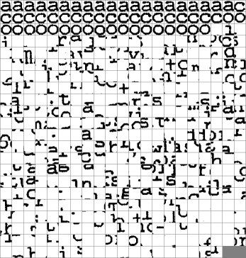
Using the exact same method I used to extract the letter e, I manually extracted 20 instances for each of the letters 'c','o', and 'a' since these letters appear to have features in common with the letter e, making them difficult to distinguish in some cases. I then took the images without the letter 'e' in them and ran I matlab script I wrote to automatically find and extract 400 random 32x32 areas from the e-less images. I now had my negative training set, meaning they are examples of what the letter 'e' should not look like.

Creating the Filters for the Weak Classifiers
Before I can create a group of Bayes classifiers to run through Adaboost, Each classifier needs to have a filter. Each filter does not have to be very good (in fact, if it is too good it might affect the results of Adaboost negatively) but it should yield a response that will be classified as correct for more than 50% of the time. A classifier that is correct exactly 50% of the time means that it randomly guesses if the image it is testing is a letter 'e'. One question that may arise would be "how do you know how to generate a filter that will work well with Adaboost?". The answer is basically "you don't have to". This is because Adaboost will automatically determine which filters are the best by measuring the accuracy of each weak classifier corresponding to each filter. So, in order to allow Adaboost to select effective filters, the trick is to choose "quantity" over "quality". Each filter should concentrate on a small area of the image and should be fast to compute. Initially, I generated about 7800 different filters where the sum of certain areas of the filter are subtracted from the sum of the other areas of the filter. This is done by setting some pixels to be -1 and others to be 1. When each 32x32 pixel filter is convolved with a 32x32 pixel image, this yields the same result. Dlagnekov did the same thing in his paper, but he used an optimization technique called integral images so that he would not have to compute the sum of every pixel region every time --the sum at different rectangular areas of each image is precomputed and stored. The 7800 filters that I generated didn't seem to work very well. Some of the filters I made consisted of a 2x2 pixel square moved at all possible image locations but these filters didn't seem to yield distinctive responses between the positive images and negative images. So, I looked at two research papers on generating filters using Haar-like features. This basically means that they took the difference between different regions like I did but they used larger-sized rectangles that were evenly divided into between 2 and 4 regions before their sums were subtracted. I decided to create a new Matlab script to generate a new set of filters that more closely resemble Haar-like features:

To generate this set of filters, I opened up an image of the letter 'e' in a photo-editor called Gimp and tried to identify regions of the letter 'e' that might yield a good classification. I figured that the following colored regions might be areas with good features:

The region to the right measures to be around 16x8 pixels, so I generated filters where all pixels were black except for a single 16x8 region where half of the pixels had value 1 and the other half had value -1.
Creating a Bayes Weak Classifier
In order to turn a particular filter into a Bayes classifier, there are 3 main steps that should be taken:
1) convolve the filter with all negative and positive training images and generate a separate histogram for each. Set the range of each histogram to be from the minimum value of both positive and negative responses to the maximum value of these responses. L1 Normalize each histogram by dividing the height of each bin by the sum of all of the bins. This will make the sum of each histogram add up to 1.
2) find the prior probability of finding the letter 'e' and the prior probability of finding a letter other than e. This means "if I pick a letter at random from a random piece of paper, what are the odds that the letter I pick is the letter 'e' ?". I asked my professor about this and he searched Google to come up with a probability of about 12% of finding the letter 'e'. The probability of finding a letter other than e is 100-12 = 88%.
3) find the mean and standard deviation of each set of responses, before they are binned into the histogram
When all 3 of these steps are done, the values generated are plugged into an equation that will basically fit a gaussian curve to each histogram, resulting in two humps.
The equation to use is:
(1 / ( sqrt(2*pi)*s)) * p * e^ - ( ((x-m)^2)/(2*s^2) )
where s,m is the standard deviation and mean from step 3, p is the prior probability from step 2, and x is the values of the x-axis of each histogram (ie: the values of the filter responses used to set the histogram bins).
When the two curves are generated, a cutoff point is set where anything to one side of the cutoff point is considered to be an 'e' and anything to the other side is considered to not be an 'e'. If a classifier is effective, then when the response of a new image is taken with the classifier's filter, this response should fall to the correct side of the cutoff point. If it falls to the side marked by the positive responses, then the image in question is considered to be the letter 'e' and "true" is returned. Otherwise, "false" is returned.
Generating Responses
When I graphed the response of a particular filter where a 16x8 pixel region was located on the right side, I got two curves completely inside each other. This is completely the opposite of what I thought would happen. I thought that since the right side of the letter 'e' looks different than the letters c,o, and a, then a filter with a 16x8 pixel window here would generate good responses. I wanted to make sure that at least some of my filters were good before I tried to run Adaboost on them. Otherwise, I would not know if Adaboost was working well or not. I talked with my professor and he suggested that I generate Bayes classifiers for each curve, calculate the error for each classifier, and determine which classifiers have the lowest error. The filters that perform the best will yield classifiers with the lowest calculated error. This way, I can reliably determine which curves have the lowest error rates and thus the best classification rates. This will provide a way to gauge the effectiveness of Adaboost as well as the quality of my generated filters.

Papers Reffered to
/*frequency of letter e*/
http://cm.bell-labs.com/cm/ms/what/shannonday/shannon1948.pdf
/*Haar-like features*/
http://citeseer.ist.psu.edu/viola01rapid.html
http://citeseer.ist.psu.edu/mohan01examplebased.html
/*dot-matrix scanned paper for training set*/
http://www-cse.ucsd.edu/classes/sp02/cse252/foerstner/foerstner.pdf
I wrote up a trivial example of generating a training set and applying classifiers on paper, but I wasn't getting a nice looking graph with two distinct humps. Instead, I was getting an almost flat curve for the positive training set and two impulses for the negative training set. I talked with my professor and he said that the type of classifiers Dlagnekov uses are statistical classifiers, meaning that in order to get good curves, one must have a large number of positive and negative classifiers. He suggested that I implement an Adaboost method for detecting the letter "e" (lowercase) on a white sheet of paper before attempting to detect soda cans. He provided me with a link to a research paper that was first printed out with a dot-matrix printer, then scanned in and converted to PDF format. This means that the letters in the paper vary quite a bit, making the detection process nontrivial. He suggested that I use this paper to generate positive and negative training examples as well as using it to test my implementation. Here is a link to the paper I used:
http://www-cse.ucsd.edu/classes/sp02/cse252/foerstner/foerstner.pdf
Creating the Positive Training Set
I wanted each image to be 32x32 pixels so I zoomed in with Adobe Reader to a 400% scale and took a screenshot. I then pasted the screenshot into Windows Paintbrush and manually cut out every lowercase "e" in the image. I repeated this process until I had 100 different lowercase "e"s in a single bitmap image. This image was then run through a Matlab script I wrote where, when I click the center of each letter 'e', a 32x32 pixel region surrounding the selected location is automatically exported as a new bitmap file. I also saved the image with every lowercase "e" removed so I could later use this e-less image to create negative training examples. Since the research paper was scanned-in with a dot-matrix printer, the quality of each letter e is slightly different --some e's are almost perfect while others look more like o's. These images make up my positive training set, meaning they are examples of what the letter 'e' should look like. Here is a composite image consisting of all of the 32x32 images of the letter 'e' created for visualization purposes using a matlab script:
Creating the Negative Training Set
Using the exact same method I used to extract the letter e, I manually extracted 20 instances for each of the letters 'c','o', and 'a' since these letters appear to have features in common with the letter e, making them difficult to distinguish in some cases. I then took the images without the letter 'e' in them and ran I matlab script I wrote to automatically find and extract 400 random 32x32 areas from the e-less images. I now had my negative training set, meaning they are examples of what the letter 'e' should not look like.
Creating the Filters for the Weak Classifiers
Before I can create a group of Bayes classifiers to run through Adaboost, Each classifier needs to have a filter. Each filter does not have to be very good (in fact, if it is too good it might affect the results of Adaboost negatively) but it should yield a response that will be classified as correct for more than 50% of the time. A classifier that is correct exactly 50% of the time means that it randomly guesses if the image it is testing is a letter 'e'. One question that may arise would be "how do you know how to generate a filter that will work well with Adaboost?". The answer is basically "you don't have to". This is because Adaboost will automatically determine which filters are the best by measuring the accuracy of each weak classifier corresponding to each filter. So, in order to allow Adaboost to select effective filters, the trick is to choose "quantity" over "quality". Each filter should concentrate on a small area of the image and should be fast to compute. Initially, I generated about 7800 different filters where the sum of certain areas of the filter are subtracted from the sum of the other areas of the filter. This is done by setting some pixels to be -1 and others to be 1. When each 32x32 pixel filter is convolved with a 32x32 pixel image, this yields the same result. Dlagnekov did the same thing in his paper, but he used an optimization technique called integral images so that he would not have to compute the sum of every pixel region every time --the sum at different rectangular areas of each image is precomputed and stored. The 7800 filters that I generated didn't seem to work very well. Some of the filters I made consisted of a 2x2 pixel square moved at all possible image locations but these filters didn't seem to yield distinctive responses between the positive images and negative images. So, I looked at two research papers on generating filters using Haar-like features. This basically means that they took the difference between different regions like I did but they used larger-sized rectangles that were evenly divided into between 2 and 4 regions before their sums were subtracted. I decided to create a new Matlab script to generate a new set of filters that more closely resemble Haar-like features:
To generate this set of filters, I opened up an image of the letter 'e' in a photo-editor called Gimp and tried to identify regions of the letter 'e' that might yield a good classification. I figured that the following colored regions might be areas with good features:

The region to the right measures to be around 16x8 pixels, so I generated filters where all pixels were black except for a single 16x8 region where half of the pixels had value 1 and the other half had value -1.
Creating a Bayes Weak Classifier
In order to turn a particular filter into a Bayes classifier, there are 3 main steps that should be taken:
1) convolve the filter with all negative and positive training images and generate a separate histogram for each. Set the range of each histogram to be from the minimum value of both positive and negative responses to the maximum value of these responses. L1 Normalize each histogram by dividing the height of each bin by the sum of all of the bins. This will make the sum of each histogram add up to 1.
2) find the prior probability of finding the letter 'e' and the prior probability of finding a letter other than e. This means "if I pick a letter at random from a random piece of paper, what are the odds that the letter I pick is the letter 'e' ?". I asked my professor about this and he searched Google to come up with a probability of about 12% of finding the letter 'e'. The probability of finding a letter other than e is 100-12 = 88%.
3) find the mean and standard deviation of each set of responses, before they are binned into the histogram
When all 3 of these steps are done, the values generated are plugged into an equation that will basically fit a gaussian curve to each histogram, resulting in two humps.
The equation to use is:
(1 / ( sqrt(2*pi)*s)) * p * e^ - ( ((x-m)^2)/(2*s^2) )
where s,m is the standard deviation and mean from step 3, p is the prior probability from step 2, and x is the values of the x-axis of each histogram (ie: the values of the filter responses used to set the histogram bins).
When the two curves are generated, a cutoff point is set where anything to one side of the cutoff point is considered to be an 'e' and anything to the other side is considered to not be an 'e'. If a classifier is effective, then when the response of a new image is taken with the classifier's filter, this response should fall to the correct side of the cutoff point. If it falls to the side marked by the positive responses, then the image in question is considered to be the letter 'e' and "true" is returned. Otherwise, "false" is returned.
Generating Responses
When I graphed the response of a particular filter where a 16x8 pixel region was located on the right side, I got two curves completely inside each other. This is completely the opposite of what I thought would happen. I thought that since the right side of the letter 'e' looks different than the letters c,o, and a, then a filter with a 16x8 pixel window here would generate good responses. I wanted to make sure that at least some of my filters were good before I tried to run Adaboost on them. Otherwise, I would not know if Adaboost was working well or not. I talked with my professor and he suggested that I generate Bayes classifiers for each curve, calculate the error for each classifier, and determine which classifiers have the lowest error. The filters that perform the best will yield classifiers with the lowest calculated error. This way, I can reliably determine which curves have the lowest error rates and thus the best classification rates. This will provide a way to gauge the effectiveness of Adaboost as well as the quality of my generated filters.

Papers Reffered to
/*frequency of letter e*/
http://cm.bell-labs.com/cm/ms/what/shannonday/shannon1948.pdf
/*Haar-like features*/
http://citeseer.ist.psu.edu/viola01rapid.html
http://citeseer.ist.psu.edu/mohan01examplebased.html
/*dot-matrix scanned paper for training set*/
http://www-cse.ucsd.edu/classes/sp02/cse252/foerstner/foerstner.pdf
Subscribe to:
Posts (Atom)