Here is an example of my second scale strong classifier running on some video footage.
It seems to do well towards the middle where there is little background clutter and the
soda cans are about the size of the detection rectangle. I will have to do something
about those false positives though.
NOTE: this video requires a divx decoder even though it is in WMV format.
http://members.cox.net/fbirchmore/testcan-2_1.5.wmv
Thursday, March 23, 2006
Wednesday, March 22, 2006
Final Powerpoint Presentation
Here is a link to a PDF of my final powerpoint presentation:
http://members.cox.net/fbirchmore/cse%20190a/soda_cans.pdf
http://members.cox.net/fbirchmore/cse%20190a/soda_cans.pdf
Saturday, March 11, 2006
Detecting Soda Cans Using C++
I have successfully migrated from my Matlab implementation to Louka's C++ code for recognizing license plates. I have been having all sorts of problems getting his code to compile on my laptop. Fortunately, the code is running on Greg's computer so I finally resorted to using ssh to log into his computer in order to run Louka's code.
The C++ implementation works by reading in a text file where each line of the text file specifies the name of an image followed by the bounding box coordinates of a license plate in the image. Here is an example:
images/image1.jpg 20,20,80,80
This means that in the image "image1.jpg" in the directory "images", there is a license plate in that image with the upper-left corner at (20,20) and the lower-right corner at (80,80). Interestingly, negative training examples (ie: "not a license plate") are acquired by randomly selecting areas that do not overlap with the bounding boxes of the license plates. Unlike my method for training my Matlab implementation, background images can be obtained from areas immediately surrounding license plate locations. In my Matlab implementation for detecting soda cans, cropped images with soda cans removed have to be fed in to extract negative training examples --meaning that the areas immediately surrounding soda cans may yield a large number of false positive classifications (ie: detecting background clutter as a soda can). Another very important advantage to Louka's implementation is that areas containing soda cans can be of ALL DIFFERENT SIZES since a large detection window can overlap with the background. In addition, the quality of a detection can be determined by offsetting the bounding boxes for some of the training images and adding these offset images as additional positive training examples--causing "good" detections to be recognized by the presence of many different rectangles in the areas surrounding a detected object (as Louka did in his thesis).
Modifying Louka's C++ Code to Accomodate Soda Cans
Instead of rebuilding my entire training set of soda cans using a different method, I decided to start by modifying Louka's code to accomodate my training set. After modification, his code treated each positive input image as containing only a single object to be detected. Negative examples were extracted by randomly extracting portions of a seprately specified set of images containing only background (as in my Matlab implementation). I created each list of image filenames and bounding boxes by creating a Matlab script that reads all of the images in a directory, obtains their dimensions, and outputs them to a text file.
Training the Soda Can Detector using Louka's C++ code
I initially provided 127 images of soda cans and randomly extracted 1000 background images. For this test, all soda cans and background images had the same pixel dimensions of 22 x 36. I trained a strong classifier using about 2000 filters generated by Louka for 14 rounds. I was astonished to see that it finished training in only a few minutes!! I tried increasing the number of negative examples to 1000, 10000, and 17000. Even with these large numbers of negative examples, training finished in less than an hour for each! With my Matlab implementation, training on 127 soda can images and 1000 background images took 24 hours. I believe the enormous difference in training time can be partially attributed to the fact that Matlab runs through Java and that "for" loops are slow. Matlab is designed to perform matrix calculations efficiently but I mostly used "for" loops and cell arrays. In my Matlab implementation, I also used around 7000 filters while Louka used about 2000 filters. Louka also uses a Cascade of classifiers to optimize both his training and his detection time --though only one layer was used to train the aforementioned set of images in less than an hour.
Cascade of Classifiers
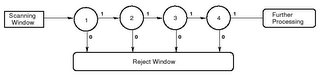
The Cascade optimization technique invloves training N layers where each layer represents a group of weak classifiers selected by Adaboost. The first layer is trained using all positive and negative training examples (ie: soda cans and non-soda cans). Each layer thereafter is trained with only the false positives (ie: background images classified as soda cans) used as the negative examples. This allows the early stages of the classifier to reject a majority of the windows immediately with only images of soda cans going through all layers of the cascade. In a typical input image, only a very small portion of the window will contain soda cans. Although an image classified as a soda can must travel through all stages of the cascade (which takes longer than a single strong classifier for this particular image) to be classified correctly, most areas of the image will be rejected immediately. If, for example, an input image contained a single soda can against a very sparse background, then the area containing the soda can would be run through all layers of the Cascade while the other areas of the image might only be run through a single layer. This results in a much faster training time and detection time at the expense of a higher number of false positives at later stages of the Cascade. To reduce the number of false positives, the later stages of the Cascade require a larger number of weak classifiers. Here is a diagram from Louka's paper illustrating how a Cascade works:
Detection Results
After I trained a single-stage classifier using 127 positive and about 17000 negative images with a single scale of soda can (22x36 pixels), the resulting strong classifier classified all 10 test images correctly. However, when I ran the same classifier on the same input image shown in my previous blog post, my detection rate was much lower. I decided that if I want to train a multiple layer cascade and use multiple scales, I would have to revert to Louka's original C++ implementation and rebuild my training set to fit this structure.
Rebuilding the Training Set
I decided that this time I would not try to build an image annotation toolset from scratch as I did with the letter 'e'. I explored the internet and found that the popular online annotation tool "LabelMe" has a Matlab toolbox:
http://people.csail.mit.edu/torralba/LabelMeToolbox/
I also discovered that they have an object recognition algorithm written in Matlab using "GentleBoost" which is a variation of Adaboost.
ttp://people.csail.mit.edu/torralba/iccv2005/boosting/boosting.html
However, I decided not to use this toolbox because their output format is XML when I wanted a normal textfile (I found out later that this would have been alright). I searched the internet some more and came across an annotation toolset:
http://www.pascal-network.org/challenges/VOC/voc2005/
This toolset will cycle through all images in a directory and let the user draw bounding boxes around the objects in the scene. The objects are then manually assigned a label. I created four different labels for four different types of pepsi cans that can be described as follows:
1 = upright, unoccluded pepsi can
2 = upright, partially occluded pepsi can
3 = horizontal, unoccluded pepsi can
4 = horizontal, partially occluded pepsi can
I then went through all of the same images from which I extracted my original training set and drew a bounding box around each pepsi can in the image. Next, I wrote a Matlab script to read in all of these extracted objects and export their names and bounding boxes to a single text file in a format recognizable by Louka's C++ code. I then converted the bounding box portions into a CSV file and loaded it into OpenOffice Calc so I could organize these coordinates into different scales etc. I decided to find the largest bounding box and use this size as the window for my strong classifier. Unlike my first training set which took about 7 hours to create, this training set took only a few hours to create and is much more useful. I labeled a total of 698 soda cans at a variety of different scales. Here is an example of one of the annotated images:

Notice that another of SPAWAR's robots, called the ATRV, has been used to clutter the background of the soda cans. This robot has a variety of detail with which to test the performance of my soda can detection algorithm as well as enforce Robart III's ability to avoid targeting a fellow robot.
I then trained a strong classifier using all 698 soda can images and about 6000 negative examples.
I will find out if this classifier was trained or not on monday.
The Next Step
The next step will be to once again organize the soda can images into different scales only this time the images will not be cropped and only the detection window will be scaled (the bounding boxes will not be modified). I will also add additional layers to the cascade of each image size. Although Louka mentioned in his thesis that license plate detection rates were not as high when input images were scaled in a pyramid, I may try this approach for soda cans just to see what happens.
The C++ implementation works by reading in a text file where each line of the text file specifies the name of an image followed by the bounding box coordinates of a license plate in the image. Here is an example:
images/image1.jpg 20,20,80,80
This means that in the image "image1.jpg" in the directory "images", there is a license plate in that image with the upper-left corner at (20,20) and the lower-right corner at (80,80). Interestingly, negative training examples (ie: "not a license plate") are acquired by randomly selecting areas that do not overlap with the bounding boxes of the license plates. Unlike my method for training my Matlab implementation, background images can be obtained from areas immediately surrounding license plate locations. In my Matlab implementation for detecting soda cans, cropped images with soda cans removed have to be fed in to extract negative training examples --meaning that the areas immediately surrounding soda cans may yield a large number of false positive classifications (ie: detecting background clutter as a soda can). Another very important advantage to Louka's implementation is that areas containing soda cans can be of ALL DIFFERENT SIZES since a large detection window can overlap with the background. In addition, the quality of a detection can be determined by offsetting the bounding boxes for some of the training images and adding these offset images as additional positive training examples--causing "good" detections to be recognized by the presence of many different rectangles in the areas surrounding a detected object (as Louka did in his thesis).
Modifying Louka's C++ Code to Accomodate Soda Cans
Instead of rebuilding my entire training set of soda cans using a different method, I decided to start by modifying Louka's code to accomodate my training set. After modification, his code treated each positive input image as containing only a single object to be detected. Negative examples were extracted by randomly extracting portions of a seprately specified set of images containing only background (as in my Matlab implementation). I created each list of image filenames and bounding boxes by creating a Matlab script that reads all of the images in a directory, obtains their dimensions, and outputs them to a text file.
Training the Soda Can Detector using Louka's C++ code
I initially provided 127 images of soda cans and randomly extracted 1000 background images. For this test, all soda cans and background images had the same pixel dimensions of 22 x 36. I trained a strong classifier using about 2000 filters generated by Louka for 14 rounds. I was astonished to see that it finished training in only a few minutes!! I tried increasing the number of negative examples to 1000, 10000, and 17000. Even with these large numbers of negative examples, training finished in less than an hour for each! With my Matlab implementation, training on 127 soda can images and 1000 background images took 24 hours. I believe the enormous difference in training time can be partially attributed to the fact that Matlab runs through Java and that "for" loops are slow. Matlab is designed to perform matrix calculations efficiently but I mostly used "for" loops and cell arrays. In my Matlab implementation, I also used around 7000 filters while Louka used about 2000 filters. Louka also uses a Cascade of classifiers to optimize both his training and his detection time --though only one layer was used to train the aforementioned set of images in less than an hour.
Cascade of Classifiers
The Cascade optimization technique invloves training N layers where each layer represents a group of weak classifiers selected by Adaboost. The first layer is trained using all positive and negative training examples (ie: soda cans and non-soda cans). Each layer thereafter is trained with only the false positives (ie: background images classified as soda cans) used as the negative examples. This allows the early stages of the classifier to reject a majority of the windows immediately with only images of soda cans going through all layers of the cascade. In a typical input image, only a very small portion of the window will contain soda cans. Although an image classified as a soda can must travel through all stages of the cascade (which takes longer than a single strong classifier for this particular image) to be classified correctly, most areas of the image will be rejected immediately. If, for example, an input image contained a single soda can against a very sparse background, then the area containing the soda can would be run through all layers of the Cascade while the other areas of the image might only be run through a single layer. This results in a much faster training time and detection time at the expense of a higher number of false positives at later stages of the Cascade. To reduce the number of false positives, the later stages of the Cascade require a larger number of weak classifiers. Here is a diagram from Louka's paper illustrating how a Cascade works:

Detection Results
After I trained a single-stage classifier using 127 positive and about 17000 negative images with a single scale of soda can (22x36 pixels), the resulting strong classifier classified all 10 test images correctly. However, when I ran the same classifier on the same input image shown in my previous blog post, my detection rate was much lower. I decided that if I want to train a multiple layer cascade and use multiple scales, I would have to revert to Louka's original C++ implementation and rebuild my training set to fit this structure.
Rebuilding the Training Set
I decided that this time I would not try to build an image annotation toolset from scratch as I did with the letter 'e'. I explored the internet and found that the popular online annotation tool "LabelMe" has a Matlab toolbox:
http://people.csail.mit.edu/torralba/LabelMeToolbox/
I also discovered that they have an object recognition algorithm written in Matlab using "GentleBoost" which is a variation of Adaboost.
ttp://people.csail.mit.edu/torralba/iccv2005/boosting/boosting.html
However, I decided not to use this toolbox because their output format is XML when I wanted a normal textfile (I found out later that this would have been alright). I searched the internet some more and came across an annotation toolset:
http://www.pascal-network.org/challenges/VOC/voc2005/
This toolset will cycle through all images in a directory and let the user draw bounding boxes around the objects in the scene. The objects are then manually assigned a label. I created four different labels for four different types of pepsi cans that can be described as follows:
1 = upright, unoccluded pepsi can
2 = upright, partially occluded pepsi can
3 = horizontal, unoccluded pepsi can
4 = horizontal, partially occluded pepsi can
I then went through all of the same images from which I extracted my original training set and drew a bounding box around each pepsi can in the image. Next, I wrote a Matlab script to read in all of these extracted objects and export their names and bounding boxes to a single text file in a format recognizable by Louka's C++ code. I then converted the bounding box portions into a CSV file and loaded it into OpenOffice Calc so I could organize these coordinates into different scales etc. I decided to find the largest bounding box and use this size as the window for my strong classifier. Unlike my first training set which took about 7 hours to create, this training set took only a few hours to create and is much more useful. I labeled a total of 698 soda cans at a variety of different scales. Here is an example of one of the annotated images:
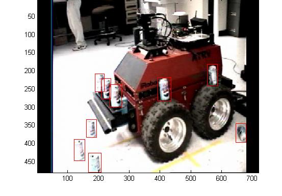
Notice that another of SPAWAR's robots, called the ATRV, has been used to clutter the background of the soda cans. This robot has a variety of detail with which to test the performance of my soda can detection algorithm as well as enforce Robart III's ability to avoid targeting a fellow robot.
I then trained a strong classifier using all 698 soda can images and about 6000 negative examples.
I will find out if this classifier was trained or not on monday.
The Next Step
The next step will be to once again organize the soda can images into different scales only this time the images will not be cropped and only the detection window will be scaled (the bounding boxes will not be modified). I will also add additional layers to the cascade of each image size. Although Louka mentioned in his thesis that license plate detection rates were not as high when input images were scaled in a pyramid, I may try this approach for soda cans just to see what happens.
Monday, March 06, 2006
Testing Soda Can Recognition
This week, I modified the letter 'e' algorithm so that soda cans can be detected. I updated my Adaboost implementation by storing filters and detecting images using HSV channels (hue, saturation, value) instead of simply grayscale or RGB. With HSV, the value channel can be filtered to achieve the same results as filtering a grayscale image. If I choose to later add color filtering, I can simply take the other two channels into account. Here is a link to the Wikipedia entry for HSV:
http://en.wikipedia.org/wiki/HSV_color_space
New Filter Types
In addition to adding HSV filtering capabilities, I also added additional types of filters. These filter types are the same that were used by Dlagnekov in his LPR/MMR paper. The new types of filters use Haar-like features as before only they operate on derivatives and variance instead of simply pixel values. The types of filters added include: X-derivative, Y-derivative, X-derivative-variance, Y-derivative-variance. Each different filter type is assigned a number which is stored with each filter (ie: X-derivative = 3). If a filter is known to operate on the X-derivative of an image and this particular filter consists of "1"s in the top-half and "0"s in the bottom half, then the sum of the pixels in the bottom-half of the X-derivative of an image will effectively be subtracted from the top-half. To get the X derivative of an image, a Sobel kernel is convolved with the input image at each pixel location. This is accomplished by calling the matlab function 'conv2' with the input image and a Sobel kernel created with 'fspecial' as arguments. Here are the links to the Matlab help pages for these two functions:
http://www.mathworks.com/access/helpdesk/help/toolbox/images/fspecial.html
http://www.mathworks.com/access/helpdesk/help/techdoc/ref/conv2.html
Filters Generated
For my inital soda can classifier, I chose to use only one scale of training images --size category 2 (22 x 36 pixels). To detect soda cans at this scale, I generated a new set of filters that I thought would work well for detecting features of these soda cans. I generated three different categories of filters of sizes 22 x 36, 22 x 8, and 16 x 16. My intent was that the 22 x 8 filter would extract features from the top and sides of the soda can and the 16 x 16 filter would extract features from the corners and the logo. For each of these filter sizes, I generated 7 different types of feature computation that add/subtract values from the pixel intensities of the following:
1. original image
2. x-derivative image
3. x-derivative-squared image
4. x-derivative variance
5. y-derivative image
6. y-derivative-squared image
7. y-derivative variance
The squared derivatives were computed so that the variance could easily be obtained
but I decided to generate separate groups of filters for them just to see what happens.
Test Results
Using the aforementioned configuration, I trained Adaboost for 20 rounds using 127 images of 22 x 36 soda cans (positive training images) and 480 images of 22 x 36 random background (negative training images). Training took an unreasonably long time of about 8 hours. This is probably due to the fact that I am calculating the derivative of each image as I obtain their filter responses. This can be fixed by precomputing the derivatives of the training images which will probably result in a dramatic increase in both training and testing efficiency.
After Adaboost finished training, the detection rates for the test images looked pretty good with classification rates of 95.2224% with the remaining 4.777% due to false negatives (ie: it is a soda can but was not classified as one). These results were obtained from testing 10 positive and 20 negative training images that were removed from the training set prior to running Adaboost. However, after running the strong classifier on a full image that was scaled to 70% (so soda cans are around 22 x 36 pixels) the results were not nearly as good:

I think that the false positives appearing around the tires may be attributed to not using enough negative training examples (background examples). I tried re-training the same strong classifier using 1000 negative examples. This took about 24 hours and yielded results that were not much better. Dlagnekov reports that he used about 10,000 negative training examples. Since I am not willing to wait a week to train a new strong classifier, the next step will be to implement the Integral Images acceleration structure (as Dlagnekov did) and precompute the image derivatives.
Integral Images (in progress)
I have currently finished implementing Integral Images and have precomputed the image derivatives. Once my implementation is working, I will re-train my classifier and hopefully achieve better and faster results.
http://en.wikipedia.org/wiki/HSV_color_space
New Filter Types
In addition to adding HSV filtering capabilities, I also added additional types of filters. These filter types are the same that were used by Dlagnekov in his LPR/MMR paper. The new types of filters use Haar-like features as before only they operate on derivatives and variance instead of simply pixel values. The types of filters added include: X-derivative, Y-derivative, X-derivative-variance, Y-derivative-variance. Each different filter type is assigned a number which is stored with each filter (ie: X-derivative = 3). If a filter is known to operate on the X-derivative of an image and this particular filter consists of "1"s in the top-half and "0"s in the bottom half, then the sum of the pixels in the bottom-half of the X-derivative of an image will effectively be subtracted from the top-half. To get the X derivative of an image, a Sobel kernel is convolved with the input image at each pixel location. This is accomplished by calling the matlab function 'conv2' with the input image and a Sobel kernel created with 'fspecial' as arguments. Here are the links to the Matlab help pages for these two functions:
http://www.mathworks.com/access/helpdesk/help/toolbox/images/fspecial.html
http://www.mathworks.com/access/helpdesk/help/techdoc/ref/conv2.html
Filters Generated
For my inital soda can classifier, I chose to use only one scale of training images --size category 2 (22 x 36 pixels). To detect soda cans at this scale, I generated a new set of filters that I thought would work well for detecting features of these soda cans. I generated three different categories of filters of sizes 22 x 36, 22 x 8, and 16 x 16. My intent was that the 22 x 8 filter would extract features from the top and sides of the soda can and the 16 x 16 filter would extract features from the corners and the logo. For each of these filter sizes, I generated 7 different types of feature computation that add/subtract values from the pixel intensities of the following:
1. original image
2. x-derivative image
3. x-derivative-squared image
4. x-derivative variance
5. y-derivative image
6. y-derivative-squared image
7. y-derivative variance
The squared derivatives were computed so that the variance could easily be obtained
but I decided to generate separate groups of filters for them just to see what happens.
Test Results
Using the aforementioned configuration, I trained Adaboost for 20 rounds using 127 images of 22 x 36 soda cans (positive training images) and 480 images of 22 x 36 random background (negative training images). Training took an unreasonably long time of about 8 hours. This is probably due to the fact that I am calculating the derivative of each image as I obtain their filter responses. This can be fixed by precomputing the derivatives of the training images which will probably result in a dramatic increase in both training and testing efficiency.
After Adaboost finished training, the detection rates for the test images looked pretty good with classification rates of 95.2224% with the remaining 4.777% due to false negatives (ie: it is a soda can but was not classified as one). These results were obtained from testing 10 positive and 20 negative training images that were removed from the training set prior to running Adaboost. However, after running the strong classifier on a full image that was scaled to 70% (so soda cans are around 22 x 36 pixels) the results were not nearly as good:
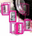
I think that the false positives appearing around the tires may be attributed to not using enough negative training examples (background examples). I tried re-training the same strong classifier using 1000 negative examples. This took about 24 hours and yielded results that were not much better. Dlagnekov reports that he used about 10,000 negative training examples. Since I am not willing to wait a week to train a new strong classifier, the next step will be to implement the Integral Images acceleration structure (as Dlagnekov did) and precompute the image derivatives.
Integral Images (in progress)
I have currently finished implementing Integral Images and have precomputed the image derivatives. Once my implementation is working, I will re-train my classifier and hopefully achieve better and faster results.
Subscribe to:
Posts (Atom)