Testing Soda Can Recognition

This week, I modified the letter 'e' algorithm so that soda cans can be detected. I updated my Adaboost implementation by storing filters and detecting images using HSV channels (hue, saturation, value) instead of simply grayscale or RGB. With HSV, the value channel can be filtered to achieve the same results as filtering a grayscale image. If I choose to later add color filtering, I can simply take the other two channels into account. Here is a link to the Wikipedia entry for HSV:
http://en.wikipedia.org/wiki/HSV_color_space

New Filter Types

In addition to adding HSV filtering capabilities, I also added additional types of filters. These filter types are the same that were used by Dlagnekov in his LPR/MMR paper. The new types of filters use Haar-like features as before only they operate on derivatives and variance instead of simply pixel values. The types of filters added include: X-derivative, Y-derivative, X-derivative-variance, Y-derivative-variance. Each different filter type is assigned a number which is stored with each filter (ie: X-derivative = 3). If a filter is known to operate on the X-derivative of an image and this particular filter consists of "1"s in the top-half and "0"s in the bottom half, then the sum of the pixels in the bottom-half of the X-derivative of an image will effectively be subtracted from the top-half. To get the X derivative of an image, a Sobel kernel is convolved with the input image at each pixel location. This is accomplished by calling the matlab function 'conv2' with the input image and a Sobel kernel created with 'fspecial' as arguments. Here are the links to the Matlab help pages for these two functions:
http://www.mathworks.com/access/helpdesk/help/toolbox/images/fspecial.html
http://www.mathworks.com/access/helpdesk/help/techdoc/ref/conv2.html

Filters Generated

For my inital soda can classifier, I chose to use only one scale of training images --size category 2 (22 x 36 pixels). To detect soda cans at this scale, I generated a new set of filters that I thought would work well for detecting features of these soda cans. I generated three different categories of filters of sizes 22 x 36, 22 x 8, and 16 x 16. My intent was that the 22 x 8 filter would extract features from the top and sides of the soda can and the 16 x 16 filter would extract features from the corners and the logo. For each of these filter sizes, I generated 7 different types of feature computation that add/subtract values from the pixel intensities of the following:

1. original image
2. x-derivative image
3. x-derivative-squared image
4. x-derivative variance
5. y-derivative image
6. y-derivative-squared image
7. y-derivative variance

The squared derivatives were computed so that the variance could easily be obtained
but I decided to generate separate groups of filters for them just to see what happens.

Test Results

Using the aforementioned configuration, I trained Adaboost for 20 rounds using 127 images of 22 x 36 soda cans (positive training images) and 480 images of 22 x 36 random background (negative training images). Training took an unreasonably long time of about 8 hours. This is probably due to the fact that I am calculating the derivative of each image as I obtain their filter responses. This can be fixed by precomputing the derivatives of the training images which will probably result in a dramatic increase in both training and testing efficiency.

After Adaboost finished training, the detection rates for the test images looked pretty good with classification rates of 95.2224% with the remaining 4.777% due to false negatives (ie: it is a soda can but was not classified as one). These results were obtained from testing 10 positive and 20 negative training images that were removed from the training set prior to running Adaboost. However, after running the strong classifier on a full image that was scaled to 70% (so soda cans are around 22 x 36 pixels) the results were not nearly as good:



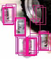
I think that the false positives appearing around the tires may be attributed to not using enough negative training examples (background examples). I tried re-training the same strong classifier using 1000 negative examples. This took about 24 hours and yielded results that were not much better. Dlagnekov reports that he used about 10,000 negative training examples. Since I am not willing to wait a week to train a new strong classifier, the next step will be to implement the Integral Images acceleration structure (as Dlagnekov did) and precompute the image derivatives.

Integral Images (in progress)

I have currently finished implementing Integral Images and have precomputed the image derivatives. Once my implementation is working, I will re-train my classifier and hopefully achieve better and faster results.