Keypoint Matching With Real Frames

I tried applying the keypoint-matching portion of the SIFT paper to an input image but I did not achieve very good results. I matched two input images to my database of several hundred different soda-can images and typically achieved results as shown in the first picture. This seems to indicate that when a cluttered background is present, matching individual keypoints does not produce reliable results. The second image shows all of the keypoints found in the input image, which is around 400. It appears that keypoints are being generated for each soda-can in the input image but these are not being determined to be the closest-matching keypoints in the scene.

In order to further determine what the problem is, I tried matching a database image with a frame containing exactly the same image of the soda can in the database. Though this is definitely not a way to test a Computer Vision algorithm for classification ability, it gave some indication about why the poor matching results were occurring. Even though the same image was used, not all of the points were matched. This indicates that analyzing the constellation of points is very important when dealing with a cluttered background. Otherwise, the background could have so much variety to it that keypoints arising in it would match better than keypoints in the correct object. Lowe describes in his SIFT paper a process of using clusters of results from a generalized Hough Transform. Although Lowe achieved good matching results using just his keypoint matching algorithm, he used high-resolution images where the keypoints within the objects in question were numerous and apparently more distinguishable from the background, as seen with a book-matching example at this link: http://www.cs.ubc.ca/~lowe/keypoints/

The next step that I take might be to implement the generalized Hough Transform that Lowe mentions, followed by a pose-estimation. One concern I have is that there are not enough keypoints that can be matched to a database of images. In an earlier blog posting, I showed matching results from comparing high-resolution images to low-resolution images that were scaled-down and oriented differently. These results showed that sometimes there were no keypoint matches between different scales of soda cans. If I have to add many different soda-can scales as well as orientations to my database of images, then the matching algorithm might become prohibitively inefficient and the accuracy level might drop even lower.

I might try using PCA-SIFT to extract keypoints. This algorithm replaces the "smoothed-histogram" that Lowe uses in his keypoint creation stages with PCA (principal component analysis). The PCA-SIFT keypoints are supposedly better at handling noisy images but are more prone to localization error. I was also thinking about using the features described in the Video Google paper, but there is no indication as to how efficient the computation of the "visual words" is. The Video Google paper apparently assumes that the "visual words" are already computed in a video before objects are classified.

Perhaps a long-term solution to object detection using mobile robots should be to simply detect the presence of an object with no regard as to what type of object it is. Objects of a certain size, color, dimension etc. could then be inspected more closely where some SIFT variation could be applied. Perhaps eventually an entire scene could be constructed into a 3D model and while this process is taking place, some easy to recognize objects could be classified before the entire 3D reconstruction completes.

I think that for now, I will implement the generalized Hough Transform and the other stages mentioned in Lowe's SIFT paper and see under what conditions soda cans can be recognized well. I will then be able to better determine if enough keypoints are being generated. I will also be able to determine where Adaboost fits in the detection/recognition process.

Removing The Background of Training Images

I recently wrote a program to white-out the background of my soda can training images. Since I wanted to reuse the training set from my experiments with Adaboost, I had to implement two different stages to accomplish this.

The first stage involved writing a Perl script to reformat the polygon files that were created by the "Javimap" program I used. This script read all of the polygons in all of the files and merged them into a single text file. Thanks to Perl's build-in regular expression matching capabilities, this process worked quite well.

The second stage involved writing a C program to cut out each soda can subimage from the training images and white-out its background. I chose C because David Lowe's provided code is written in C and contains some functions for manipulating PGM files (which he chose for his SIFT implementation).

In order to white-out the background of the soda-can images, I checked each pixel to see if it was within the polygon that I specified when first creating the training images. To accomplish this task, I implemented an algorithm that was provided on this website for raytracing:

http://neptune.cs.byu.edu/egbert/455/CourseNotes/Lecture13-RayTracingIntersections.ppt

My entire algorithm went as follows:

1) read each polygon and load its corresponding image from the Perl-generated text file of polygon coordinates.

2) cycle through each set of polygon coordinates to find the largest and smallest pair of (x,y). Use these values to specify a bounding-box for each soda can.

3) Using the bounding box from (2), crop out the image within this bounding box (should be a single soda can).

4) Translate all polygon coordinates by subtracting the smaller bounding box coordinate from each (so they are with respect to (0,0) rather than the smaller bounding-box coordinate. This is because a new image was created with the bounding box region.)

5) For each pixel in the subimage, check if it is within the bounding polygon. If not, then set that pixel value to 1.0, which is white. To determine if a pixel is within the polygon, the polygon is translated to a new coordinate system where the pixel in question is at the origin. The edges of the polygon are then checked to see if they intersect the x-axis. If the number of intersections is odd, then the pixel is inside the polygon. If the number of intersections is even, then the pixel is not inside the polygon. More details on this algorithm can be found at the aforementioned website.

Now that I have created an algorithm to automatically extract training images with clutter-free backgrounds, I can redo the training set very easily if needed without having to manually white-out the background with Gimp.

The next step will be to proceed with matching input test images against my new database of soda-can images. I will then try applying additional concepts from the SIFT paper to filter out false-positives etc.

Learning Perl

It took me quite a while to extract the number of keypoints detected and insert them into a spreadsheet. To make future tasks easier, I decided to learn Perl scripting. I read over some tutorials and books. From what I've learned about Perl, I created a script to remove keypoints and their corresponding images from the database it the number of keypoints detected in them is less than 3. This is accomplished by parsing the output text file from detecting keypoints in the database directory. Now that I can make Perl scripts, I should be able to accomplish many tasks faster by automating the more tedious work.

Here is a sample from the output file from creating database keypoints:

extracting keypoints: ./database/s06.pgm -> ./database/s06.key
Finding keypoints...
22 keypoints found.
extracting keypoints: ./database/ss01.pgm -> ./database/ss01.key
Finding keypoints...
2 keypoints found.
extracting keypoints: ./database/ss02.pgm -> ./database/ss02.key
Finding keypoints...
3 keypoints found.
extracting keypoints: ./database/ss03.pgm -> ./database/ss03.key
Finding keypoints...
0 keypoints found.

Here is the Perl script I wrote. It is called by passing in the name of the output text file ( a sample of which is above). The # signs represent comments:
#!usr/bin/perl
my $rmkp = ">./rmkp.txt";
my $line;
my $prevLine;
#@ARGV[0]: output text filename from keypoint detection.
open ( FILE, "@ARGV[0]") or
die "Cannot open input file: @ARGV[0] : $!\n";
while( $line = ) {
# i means case insensitive
# ([^>]*) match zero or more characters but not '>'
# if line matches regexp
if( $line =~ m/extracting keypoints:([^>]*)>/ ){
#removing words
$line =~ s/extracting keypoints:([^>]*)>//g;
#remove file extension
$line =~ s/.key//g;
#remove whitespace
$line =~ s/\s//g;
#store current line
$prevLine = $line;
}
#if number of keypoints found, store number
if($line =~ m/keypoints found./){
$line =~ s/keypoints found.//g;
$line =~ s/\n//g;
#if less than 3 keypoints
if($line <>

Here is the log file, rmkp.txt, generated by the Perl script. This shows the number of keypoints for the associated keypoint and image files that were deleted:
Files Deleted From Database:

2 ./database/ss01.key ./database/ss01.pgm
0 ./database/ss03.key ./database/ss03.pgm

Analysis of Keypoint Matching

Image 1: table of keypoint matches (rows on the left matched with columns on the top)
Image 2: table of keypoints where entries with <2 or entries where an image was matched to itself were set to zero.
Image 3: a graph of the table in Image 2.

Today, I graphed the matching of keypoints. The x-axis of the graph above represents the keypoints from the input images. The y-axis represents the keypoints from the database. The colors indicate how many successful keypoint matches occurred. I removed all results that had fewer than 2 matching keypoints or results where the exact same keypoints were matched between identical images. One strange result is that certain images match very well when, for instance, "match image1 image2" is run and the same images yield no matches at all when "match image2 image1" is run. For instance, the image s05.pgm has 64 matches when matched with 04.pgm while no matches occur when 04.pgm is matched with s05.pgm. Because of s05.pgm's angle and small resolution of around 120x120 pixels, very few stable keypoints are found. In contrast, 04.pgm has a high resolution with around 400 keypoints found. It could be that s05.pgm's keypoints are very similar to each other because of the low pixel resolution of the image. When matched with the keypoints from 04.pgm, perhaps there are enough keypoints in 04.pgm that are close to the keypoints in s05.pgm that enough keypoints match to indicate a successful classification.

Though this table does not provide a complete set of test cases, it can be inferred that the higher resolution images match better with other high-resolution images than low to high, low to low, or high to low. I believe that the high number of matches between the high resolution images to s05.pgm is an anomoly and does not indicate that this particular image can reliably be compared to others.

If too many keypoints are stored in the database images, the computation time required to match new input images to these might be too great for real-time performance. Since Lowe was able to achieve good results using 600x480 pixel input images with smaller resolution training images, I will try doing the same. Now that I am more familiar with SIFT, I will re-read Lowe's SIFT paper. I will try to jump the gun and use the methods provided in Lowe's code to detect soda cans using footage from Robart III as the next step. This way, I will have a better idea about what problems arise. I will then look over Lowe's suggestions for narrowing down the range of useful keypoint matches using a Hough Transform etc.

Matching Keypoints

Today, I matched soda-can keypoints to each other. Conveniently, C-code for doing this is provided with David Lowe's Keypoint generation code. Using the above set of images, I found keypoints for each image and matched them with the keypoints from all of the other images. The images with a prefix of "s" are the images without an "s" that have been scaled down to 3% of their original size and then scaled up by 600%. The resulting images with prefix "s" are of a size of around 150x240 pixels. The other images have a size of about 1100x2100 pixels. This was done as a test to see how much of an effect the resolution of the images has on extracting keypoints, which angles have the most matchable keypoints, and if similar resolution soda-can images match better than dissimilar resolution ones. I will post the results from this small experiment along with a table and a graph on my next blog entry.

This is how keypoint matching works between two images, referred to as A and B:

1. keypoints are found in A.
2. keypoints are found in B.
3. The closest matching keypoints are found between the images. Each keypoint is a 128 dimension vector. To find the distance between two keypoints, the Euclidean distance is found between the feature vector s belonging to the keypoints. Each keypoint in A is compared with each keypoint in B by Euclidean distance to find the closest matching keypoint. A match is determined as follows:

Let a' be a point in A. Let b' and b'' be the first and second closest matching points in B to the point a'. Let D(x,y) represent the Euclidean distance between its arguments x and y.

If D(a', b')< D(a', b'')*0.6 then the closest point is chosen.
Else, no points are chosen (no matching keypoint).

According to Lowe, finding merely the closest matching keypoint does not yield a reliable match. Lowe claims that a more reliable match is determined by comparing the second-closest matching keypoint. He does this by using the second-closest matching keypoint as a threshold.

SIFT Keypoints: preliminary results

One question has arised with regards to keypoints: will soda cans in low-resolution video footage yield enough keypoints to perform SIFT effectively?

Running the Keypoint Detector

I downloaded the keypoint detection code from David Lowe's website:
http://www.cs.ubc.ca/~lowe/keypoints/

David Lowe is the creator of SIFT. The code is in binary format and was extremely easy to run in Linux. There are apparently no required libraries or dependencies to run this code. I took some photos with a digital camera and cropped out the regions containing soda cans from the background. From what I've seen so far, it appears that SIFT detects keypoints that represent characteristics within an object. I believe this means that the outline of a soda can cannot be taken into account for object detection. This may prove to be a problem if objects to be detected do not have many detailed features. To test the validity of this theory, I would like to try spray-painting a soda can a solid color and see if any SIFT keypoints are extracted. Here are some images of detected keypoints:

SCALED TO DOWN TO 1.5%:


SCALED TO DOWN TO 1.5% THEN SCALED UP TO 600%:


SCALED TO DOWN TO 3.0%:

SCALED TO DOWN TO 3.0% THEN SCALED UP TO 600%:




These cans all started out as high resolution images. These images were then scaled down to 1.5% or 3.0% of their resolution in an attempt to simulate soda cans at a typical scale encountered in live video footage. According to Lowe's README file that came with the keypoint detection code, more keypoints can be detected if an image is first scaled to a larger size. In fact, the number of detected keypoints typically doubled when a low resolution image was scaled up. The pepsi cans with a prominant logo yielded the most keypoints. The soda can in the top-most image yielded no keypoints at all. There are many cases where the specular highlights appeared to yield keypoints. These cases would be taken care of at a later stage where keypoints from different training images taken under different lighting conditions would be analyzed to determine which keypoints are invariant to scale and lighting. The more I think about it, the more appealing a hybrid solution to object detection seems --one that would incorporate data from multiple sources to arrive at a conclusion. For instance, perhaps some sort of texture recognition or color detection method could be used in conjunction with SIFT to detect objects with sparse and dense features. I will continue to investigate how SIFT can be applied to soda can detection and find out what image resolutions I have to work with. If SIFT proves to work well for objects up close, I might use some other methods to detect objects of interest and then proceed to zoom-in on those objects before applying SIFT.

The next step will be to test out keypoint matching between these detected keypoints.

New MileStones: Evaluating SIFT

I have a new set of Milestones to accomplish for this quarter. I'm very busy this quarter so I will try to accomplish as many of them as I can.

Understand SIFT thoroughly - meet by 5/10/06

The purpose of this milestone is to understand SIFT well enough to be able to set up an appropriate training set and to plan out specific implementation details. This will include locating existing SIFT-related source code and determining what software should be used (i.e. shell-scripting, ImageMagick, Matlab, OpenCV, C++ etc.). Last quarter, I implemented everything in Matlab first before attempting to implement it in C++. This quarter, I will be giving C/C++ preference and use Matlab to aid in my understanding of SIFT or to generate charts, graphs etc. I've found shell scripting to be incredibly helpful in all aspects of programming --not just for this research.

Create the Training Set - meet by 5/17/06

This will most likely involve modifying my existing training set. This training set consists of extracted images of soda cans acquired at a single scale, against a static background, under constant lightining conditions, and two separate orientations. Although the use of this training set will most likely not result in scale-invariant keypoints, it will be useful in testing other aspects of this SIFT algorithm directly against my Adaboost implementation. Invariance to background clutter, lighting, performance while in motion, and efficiency can be tested using this training set. After a working SIFT implementation is created, a training set that includes soda cans extracted under a wider variety of conditions can later be swapped with this training set. I figure that I will go through all of the steps required to apply SIFT using only a few images. Once this is done, I will have a better idea about how to create a good training set for SIFT. Last quarter, I had to redo my training set several times so I want to avoid having to do that this quarter.

Detect Keypoints- meet by 5/24/06

This will involve using a difference-of-gaussian function to search the scale-space of the soda can training images to identify scale-invariant interest points. The most stable keypoints will then be selected and assigned orientations based on their local gradient directions. These gradients will then be transformed into a representation that is resistant to shape distortion and illumination differences. This will be accomplished using an existing binary implementation, such as the version provided by David Lowe on his website. I will probably make a primitive algorithm for matching keypoints initially and then improve upon it.

Match Keypoints of New Input Images (no background clutter) - meet by 5/31/06

A database of keypoints from the training images will first be set up. A new input image will be matched with this database by finding the Euclidean distance between the feature vector of the input image and the feature vectors in the database. The new input images will include soda can images with backgrounds that have been manually removed so that no keypoints will be detected outside of the soda can regions. If background clutter is left
in, then keypoints extracted from these regions may yield so many negative classifications that false negative classifications will result even when a soda can is present in a particular region. Without background clutter, I can test keypoint matching without having to cluster the keypoints or apply any additional transformations to them.

Identify Keypoint Clusters, Apply Further Filtering of Keypoint Matches (background clutter added) - meet by 6/7/06

This will first filter correct keypoint matches from the false matches by identifying clusters of three or more keypoints that agree on the orientation, scale, and location of the detected object. This is described in Lowe’s SIFT paper with a Hough Transform offered as a solution to identifying these clusters. Next, a least-squares estimate will be applied for an affine approximation to the object pose. Further analysis can be applied, as described by Lowe, to determine the probability that a particular set of features is the object being searched for.

Run Detection Method Live - meet by 6/14/06

Once a SIFT implementation is successfully implemented, it will be tested using live video footage. Initially, I might try using the same setup that I used before with the same static background. The results from this test will be compared with my previous results based on the efficiency and accuracy of detection. Various conditions will then be changed, such as the ambient lighting. Video footage will then be tested while the camera is moving horizontally with respect to the soda cans. The complexity of the tests will be gradually increased and the results analyzed unless/until the SIFT implementation begins to perform poorly. If time permits, a new set of training images will be acquired using soda cans positioned in a variety of locations and orientations and this SIFT implementation will be retested. Depending on the availability of SIFT source code online, some of these milestones can be combined and their theoretical completion dates moved back or forward.

Testing Soda Can Detection on Robart III

http://members.cox.net/fbirchmore/goodrun.mpg
http://members.cox.net/fbirchmore/goodrun2.mpg
http://members.cox.net/fbirchmore/goodrun3.mpg


We ran my soda can detection algorithm on live video from Robart III. Apparently, the classifier I have trained is very susceptible to variations in lighting and background clutter that was not present in the training data. Regardless of the aforementioned deficiencies in this particular classifier, it does quite well at eliminating almost all of the background clutter in the center of the image (only a central portion of the window is scanned as mentioned in a previous post). These false positives could be passed to another detection method for further processing or to signal to Robart III that he should zoom in on these areas for further inspection. From the results I have observed so far, I think weak classifiers that are better at detecting unique features of soda cans would work better than the haar-like features used. I think that a SIFT-based detection method will work much better , partly because it uses keypoints that would be more invariant to changes in lighting. Investigating a SIFT-based detection method will probably be the next step I will take. Although I still need to read more about SIFT to understand it fully, I am going to investigate the possibility of incorporating Adaboost into a SIFT detection method. More information on this will appear in later blog postings.

Test Video

Here is the video test footage that is mentioned in the previous post:

http://members.cox.net/fbirchmore/attempt39_out.mpg

Success (under constrained conditions)

When I had finished extracting soda-can images for my training set, I had 410 vertical and 420 horizontal soda can images. I then randomly offset each of these images by up to 1/8 of their width and 1/4 of their height to generate a total of 4444 positive training examples of vertically-oriented soda cans and 4554 positive training examples of horizontally-oriented soda cans --as Dlagnekov did in his thesis.

I then trained two classifiers using 23200 negative training examples for each. Instead of using the entire labeled image, I constrained my negative training examples to a 161x184 pixel subwindow in the bottom-center of the image. Furthermore, I used negative training examples from video footage that contained no soda-cans to begin with --rather than extracting negative examples from labeled images that exclude areas marked as containing soda cans. The first classifier used only the vertically-oriented soda-can images with a detection-window-size of 17x27 pixels and the second classifier used only the horizontally-oriented soda-can images with a detection-window-size of 30x14 pixels. The I then modified the existing license plate detection code to read in a list of classifiers from a file and run them sequentially on the source video.

Using this new framework, I ran my detection algorithm on a sample video that I had set aside before training. This sample video footage was taken using the same background that was used to build the training set. Every soda can in the video was detected very accurately with no false-positives. The worst detection in this frame is probably the upper-left where the detection window is off-center. This is probably due to the fact that the detected locations are clustered, which might be causing surrounding detection areas to average to an off-center detection area. The next step is to test this algorithm on ROBART III using live video footage.

Building a New Training Set

Next week, a portion of my work will be submitted into our Code's SPIE conference paper. Although I have decided to explore a SIFT-based method for soda can detection, my more immediate goal is to make the most of Dlagnekov's LPR detection algorithm when applied to soda can detection. The Robotics Code at SPAWAR would like to place my soda can detection algorithm directly on Robart III to test the algorithm's efficiency and accuracy. In order to make my algorithm "Robot Friendly", I am going to refine its focus to detect soda cans at a single scale against a static background. This way, my chances of success in reducing the false positive rate and increasing the true positive rate within the next week are much greater than they are for detecting soda cans at multiple scales. Furthermore, I will limit the number of orientations to only two --upright and horizontal. This will require me to train two separate strong classifiers. By keeping my detection method simple, I will be able to place my classifier directly on Robart III without having to recompile anything as well. If this is successful and there is enough time, I will add additional functionality to my algorithm and possibly get Robart III to shoot at the soda cans he sees (using all six barrels of course).

Setting Up The Soda Cans

As illustrated in the photo above, I set up Diet Pepsi Cans on and around a wooden box. This wooden box has been featured in previous SPIE conference papers submitted by the Robotics Code at SPAWAR because it is safe for Robart III to shoot at it. Without modifying the position of the wooden box or the background, I placed the soda cans at different locations and Greg recorded each setup for 5-10 seconds using Robart III's head camera. I then rotated each soda can by about 60 degrees and Greg recorded this new setup as a separate MPEG file. This was repeated 44 times to create 44 different MPEG videos. When setting up soda cans, I tried to make sure that there was just about the same number of horizontally and vertically-oriented soda cans with which I can build my training set.

Extracting JPEG Images from MPEG Videos

I used ffmpeg to extract 1-2 JPEG files from each of the 44 MPEG videos. I used the following ffmpeg command for each MPEG video:

ffmpeg -ss 00:00:03 -t 00:00:01 -i ./

Changing my mind...again...

I've decided to use the Java program. Apparently, in order to upload images to LabelMe, the images must be placed online and a link must be emailed to
Bryan Russell and Antonio Torralba at MIT. Since I am under time constraints to meet a paper deadline next week, I am just going to use the Java program. Later, when I try a SIFT-based implementation, I may use LabelMe.

Changing my Mind...Decided to use LabelMe

I've decided to use MIT's LabelMe annotation tool to rebuild my training set. At first I was hesitant to use LabelMe because I found out that their Matlab toolbox doesn't actually let you annotate images --that must be done online. I only have one copy of Matlab which is installed on a Windows machine. At this point, I would prefer to keep everything within Linux. However, I see a definite advantage to using LabelMe in that multiple people can label a set of images simultaneously since LabelMe is an online annotation tool. This means that I don't necessarily need to sit down all by myself and label images --I can solicit help. Here is the LabelMe website:

http://people.csail.mit.edu/brussell/research/LabelMe/intro.html

Getting Java to Compile

Well, with a new Linux installation comes a new set of problems. I was initially unable to compile any Java programs short of a single file containing a single "main" function (no object definitions). I kept receiving the error message below:

javac ./Javimapper.java
java ./Javimapper
Exception in thread "main" java.lang.NoClassDefFoundError: ./Javimapper

I eventually fixed the problem by referring to the following website:

http://www.cs.princeton.edu/introcs/11hello/linux.html

Upon reading the webpage above, I simply typed in the following and I was able to compile and run the program just fine:

java -classpath ./ Javimapper

Finding an Image Annotation Program

Rebuilding the Training Set

After I lower the false positive rate on my soda can classifiers, I plan to try some sort of SIFT-based approach to detecting soda cans and other objects as well. Before attempting to lower the false positive rate, I need to rebuild the training set...again. I believe that the horizontally-oriented soda cans that I have been extracting from my training footage are throwing off my detection rate. Furthermore, I have been mistakenly training classifiers using 720x480 resolution BMP images extracted from the training MPEG movies.

At the time, I was using Adobe Premiere to extract video frames since I had not yet set up ffmpeg and it had not occurred to me to use it. In order to use Adobe Premiere, I had to convert the MPEG movies into an AVI format that was at 720x480 resolution by default. I did not notice this and mistakenly thought that the original footage was 720x480 resolution when in fact it was 320x240.

By rebuilding the training set, I will be able to use smaller sliding windows for each classifier which should reduce both the training and detection times by quite a bit. When the original footage was accidentally resized to 720x480, I believe that the pixels were blurred. It will be interesting to see how much the detection rates are affected by using unmodified 320x240 footage. The 320x240 footage probably contains a greater amount of noise. However, the 320x240 footage will also train faster with each image taking up less memory --which will probably allow me to use a greater number of negative training examples and allow more bootstrapping operations with false positives.

Since I will probably soon be applying some SIFT-based approach to soda can detection, it would be beneficial if I use bounding-polygons instead of bounding-rectangles. I think this helps SIFT to avoid mistakenly extracting features from the background and allows the spread of detected points to be exploited. With this in mind, I finally decided to create a Java GUI program that will allow the user to specify bounding polygons that will be saved into different files. I will then write some code to determine the extreme points (i.e. max x, min y; max x, max y; etc...) of the polygons and set these to be the corners of rectangular bounding boxes. I will then use these bounding boxes to retrain some strong classifiers. The polygon data can then be saved for later use with SIFT or some other algorithm that would benefit from tight-fitting polygons.

Java Program to Modify

I found this Java program online by searching for "image map java" on Google. The potential candidates for image annotation programs seemed overly complex and generally only used bounding boxes. I realized that image maps that one might find on a website would use the same sort of image annotation as "image annotation toolbox" programs. I wanted to avoid using Matlab since I am less familiar with its object-oriented features than Java and I can only use Matlab on my laptop.

Here is the program I will modify:

http://www4.vc-net.ne.jp/~klivo/mapo/javimap.htm

It seems to work extremely well --especially for a 7-year-old program. I will most likely modify it by allowing it to load all images from an entire directory and making it export bounding box data in addition to polygon data.

Getting Java to Work

I took the following steps to get Java to work on my USB Hard Drive:

1) download JDK binary from Sun's website
2) type the following:

sudo apt-get install fakeroot java-package java-common
sudo dpkg -i JDK1.5.deb
sudo update-alternatives --config java

I then picked the new Java version from the menu that appeared from the update-alternatives command. I found this information at the following website:

http://www.ubuntuforums.org/archive/index.php/t-76735.html

Fixing FFMPEG

I was having trouble compiling and running the lpr_vhook program that Stephan and Kevin created. It was unable to find the highgui portion of the OpenCV library. Greg finally got it working by linking highgui.a directly into the program instead of using the shared library files. He also linked some other files that were missing by adding them to the Makefile. Apparently, my problem was that I downloaded a newer version of ffmpeg that had new library requirements so these had to be added. The ffmpeg website had removed their .tar files so I had to use their CVS repository to get the "bleeding edge" version of ffmpeg.

I learned a few new terminal commands in Linux:

ldd : list library dependencies for a file
!ff : runs most recent command that begins with the letters "ff"
history : list all commands that were typed into the terminal and enumerate them
!# : run command from "history" that has the number #

Even though it took me a week, booting Linux from a USB drive has payed off immensely in that it eliminates the need to reconfigure each Linux environment for each computer with Linux installed.

Now, I can finally redo my training set using 320x240 resolution and excluding horizontally-oriented soda cans. I may exclude partially occluded soda cans as well.

Getting X11 to work

I had some trouble getting X11 to work when I attached my USB drive to my work computer. I was getting weird colored snow instead of graphics. After trying many different things, I finally installed the proprietary nvidia drivers instead of the open-source driver called "nv". By refererring to this website, I was able to install these drivers quite easily:

http://www.ubuntuforums.org/showthread.php?t=75074&page=4

I typed in the following instructions into a terminal window:

sudo apt-get install nvidia-glx linux-restricted-modules-$(uname -r)
sudo nvidia-glx-config enable 

It worked so I have X11 now.

Installing Linux to a USB hard drive

I recently purchased a Seagate 250GB hard drive and an Acomdata aluminum external hard drive USB/Firewire case. I use a nice Dell PC at work that only has Windows installed on it. Rather than trying to reformat and repartition this PC at work, I decided to attempt to install Ubuntu 5.10 to an external USB hard drive. This way, I can bring my own personal Linux distribution wherever I go and use it on any PC (given the motherboard supports booting from a USB device) without changing the contents of the PC's hard drive. I got this to work by following the instructions provided in this article:

http://www.ubuntuforums.org/showthread.php?t=80811

In case this Ubuntu Forum post gets deleted, I have copied and pasted the appropriate steps below. My installation experience was slightly different from the original steps mentioned in the forum --I have indicated these differences with bold,italic, light-blue text.

***********************************************************************************************
Here is what I do to successfully load UBUNTU v5.10 on my EXTERNAL USB DRIVE ...

(Step 0 ) Plug the external USB drive into the computer. Unplug all of the internal IDE hard drives.

( STEP 1 ) Instead of using "expert" mode to install, I just hit enter to start the install process (using the install CD ... NOT the live CD).

INSTALL NOTE: The installation process will ask you for some information when it starts up ...

first it will ask for your language,
then your (language) location,
then your keyboard type,
then it will detect your cdrom(s),
then it will attempt to detect your network configuration,
then it will ask you to give your PC a name (hostname),
then it detects hardware and starts up the partition phase of the install.

INSTALL NOTE: When you get to STEP 2 (the partition phase), there is a simple way to determine how the install program assigns device names to your hard drive(s). Before starting any partitioning activity in STEP 2, choose the GO BACK option in the lower left corner of this screen and then choose EXECUTE A SHELL farther down in the Ubuntu installer menu that appears. Choose CONTINUE at the next prompt. In the shell window that appears, type in fdisk -l (that is FDISK -L in all lowercase). This will give you a list of all the storage devices the installer program sees. Make a note of the device names (/dev/hd? or /dev/sd?) and then type in exit to return to the partition phase (STEP 2) of the install. (Kudos to "RyanGT" for suggesting this in post #257.)

( Step 2 ) (ignore the Step 2 below) If you have a 250GB hard drive like I do, you probably don't want Ubuntu to create 3 giant partitions that span the entire drive. In fact, you will probably want to set up separate partitions manually. I set up my partitions as follows:

Filesystem Size Used Avail Use% Mounted on Fs
/dev/sda1 122M 19M 97M 17% /boot ext3
/dev/sda2 449M 255M 171M 60% / ext3
/dev/sda3 1.5G swap swap
/dev/sda5 95M 33M 62M 35% /tmp reiserfs
/dev/sda6 1.9G 492M 1.4G 26% /var reiserfs
/dev/sda7 1.9G 33M 1.9G 2% /usr/local reiserfs
/dev/sda8 5.6G 1.6G 4.1G 29% /usr reiserfs
/dev/sda9 28G 653M 28G 3% /home reiserfs

(note: I displayed this information by later typing "df -h" in a terminal window. sda4 is not present because it represents the extended partition
of the drive where sda5 - sda9 are within sda4)

I made sure that the /boot partition was small so that it does not exceed the first 1024 cylinders at the beginning of the hard drive --which I guess would make this partition not bootable.

skip this -- ( STEP 2 ) During the partitioning phase, I let the install program format my external USB drive. (I believe UBUNTU calls this a guided partitioning ... which sets up an ext2 or ext3 partition and a swap partition for you.)

INSTALL NOTE: Look for the line during the partitioning phase that might say ... erase entire disk SCSI (0,0,0) (sda). Be careful here as some people have had problems when choosing any partitioning options that include the text "and use LVM" (Kudos to "brucetan" for sharing this in post #268.)

Feel like learning about LVM anyway? Check this link out. (Kudos to "SD-Plissken" for sharing this info.)

BE VERY CAREFUL on these screens to choose the correct SDA drive and NOT an HDA drive or you may unintentionally format another drive in your system. There is no undo button for this!

Once again ... BE 100% SURE OF THE DRIVE YOU WANT TO FORMAT!

( STEP 3 ) When the install gets to loading the GRUB bootloader ... DO NOT LET IT LOAD TO ANY OTHER DRIVE BUT THE EXTERNAL USB drive we are working with here. -- This doesn't matter since the other drives should be disconnected.

Say YES when asked if you want to install Grub to the MBR (since the USB drive is the only one connected --ignore where is says "say NO" below)
The install program will ask to load GRUB to the master boot record (MBR) of your internal hard drive (HDA). Say NO to this, and on the next screen, type in the correct path to the SDA (external USB) drive where we want to install the GRUB bootloader.
(Mine was /dev/sda [NOT sda1] ... but yours may be different depending on the number and/or types of drives in your system)

COMMENT: I loaded GRUB to sda (the bootsector of the external drive) and NOT to sda1 (which would be the first partition on the external drive).

INSTALL NOTE: at this point, the install program loads some stuff and ejects the CD ... wanting you to do a reboot.

( STEP 4 ) BE 100% SURE to leave the CD in the drive (and close the drive door) before rebooting. When the PC reboots, type in rescue (to load UBUNTU in rescue mode) ( Review REQUIREMENTS at the beginning of this guide! )

Why do we startup in rescue mode you might ask? It's because we have to edit a few files to get USB support loaded before UBUNTU actually gets going. And, we also need to change a setting in the GRUB menu file to make it work correctly.

( STEP 5 ) When the system comes back up it will ask for a partition to mount. Pick the correct mount point for your external drive from the list.
(Mine was mount /dev/discs/disc1/part1 ... but yours may be different depending on the number and/or types of drives in your system)

COMMENT: /dev/discs mount points start with disc0 (with 0 meaning the first drive in a system). So, my mount point of /dev/discs/disc1/part1 was really the second disk [disc1] (the sda drive we are working with) and the first partition [part1] on that disk.

( STEP 6 ) When it comes up to a terminal window (with RESCUE MODE in the upper left corner) and just sits there, hold down Ctrl-Alt-F2 to open another terminal window for us to do our edits in.

( STEP 7 ) Type in these lines before we start editing out files ...

mount -tproc proc /target/proc
chroot /target
su

INSTALL NOTE: I used vim to edit the files. (There is a great vim cheatsheet in pdf format available from "TimL".) It is weird to use at first until you learn what a few keys do in it. The INSERT key allows you to actually enter text where you place the cursor ... The ESC key takes you out of INSERT mode ... And hitting : x saves the file and exits out of vim. (IMPORTANT TIP ... that's a colon and a lowercase x with NO SPACE between the colon and the x)

( STEP 8 ) Run vim to edit the modules file to make sure USB support is added/loaded during UBUNTU startup ...

vim /etc/mkinitramfs/modules

Right below the last line of text, enter these lines ...

ehci-hcd
usb-storage
scsi_mod
sd_mod

Be sure to save the file changes (using : x)

COMMENT: Some PCs may need a more comprehensive list added here. Please take a look at post #181 if you are having startup issues after these edits. (Kudos to "brotorious" for his efforts on this.)

( STEP 9 ) Run vim to edit the initramfs.conf file to make sure enough time elapses for USB support to load before UBUNTU gets running ...

vim /etc/mkinitramfs/initramfs.conf

At the very top of this file, add this line which tells UBUNTU to pause for 12 seconds before starting up ...

WAIT=12 (in all caps here, not sure if necessary though)

Be sure to save the file changes (using : x)

INSTALL NOTE: Editing these two files loads the necessary commands to get USB support going so UBUNTU will recognize the external USB drive. But we still need to recompile (or recreate) the initrd.img that UBUNTU uses at startup ... so that these edits actually work.

( STEP 10 ) Recompile (recreate) the initrd.img file to include USB support from these edited files ...

mkinitramfs -o /boot/initrd.img-2.6.12-9-386 /lib/modules/2.6.12-9-386

INSTALL NOTE: When you are done with the previous step #9 (and before performing this step), you can run the "ls /lib/modules" command (without the quote marks) from a terminal window to see what kernel version number you should use for this install step. They may be using a kernel version higher than 2.6.12-9-386 that was available when I originally created this help guide. (Kudos to "Saxegaard" for bringing this to my attention in post #235.)

Note: this entire step #11 might not be necessary if you disconnected the other hard drives from the computer. You may need to edit the "device.map" file though and make sure it contains the following line:
(hd0) dev/sda
If you DO end up having to edit menu.lst, make sure you type
"grub-install /dev/sda" (without the quotes of course) to update grub.

( STEP 11 ) Edit the GRUB bootloader menu file to correct a small error that looks at the wrong drive to boot from ...

vim /boot/grub/menu.lst

Navigate down this file until you get to a section where there is a menu list (not commented out ... no #s) that has Ubuntu mentioned three times (and possibly an area mentioning Windows XP down below it, if you have XP installed on an internal drive of yours).

There is a line in these three Ubuntu menu choices that has root listed on it and probably has (hd1,0) to the right of it. We need to change this to (hd0,0) on all three of these menu choices. Why? Because according to GRUB, the external USB drive will be our first drive (hd0,0) and not our second drive (hd1,0) because we loaded GRUB on it's bootsector.

INSTALL NOTE: You will also want to change a "# groot" line in a section of your menu.lst file that may look something like this ...
## default grub root device
## e.g. groot=(hd0,0)
# groot=(hd0,3) <<< groot="(hd0,0)"> until the screen actually says to press enter). Hold down Ctrl-Alt-F1 to get back to the RESCUE MODE terminal window and type exit to reboot the system.

BE 100% SURE TO GET THE CD OUT OF THE DRIVE BEFORE UBUNTU RESTARTS

( STEP 13 ) After rebooting, UBUNTU continues to run it's install process and comes to the desktop. Use the username and password you setup earlier in the install process to get into UBUNTU


That's the process I've successfully used to install UBUNTU v5.10 on an external USB drive. I hope this helps anyone whose been wrestling with this process. Let me know if it works out for you.

DAVE

Reconnect all of your hard drives and boot up the computer. (make sure you tell your bios to boot from the USB drive)
If GRUB never loads and instead gives you an error message, then you may need to install GRUB to your main hard drive. Before doing this, try plugging in your USB drive into a different computer and see if it boots up. If you need to install GRUB to your IDE hard drive, then follow the steps in this article to trick the Ubuntu installer into skipping all steps and installing only the GRUB bootloader:

http://ubuntuforums.org/showthread.php?t=76652

You can then copy the new kernel and initrd images you created in previous steps to the IDE hard drive and add them to the boot loader. To figure this out, I simply looked at other entries listed in the bootloader and applied this format to the new kernel and initrd images.


OTHER PROBLEMS AND POTENTIAL FIXES ...

* Booting Ubuntu from Windows XP without loading GRUB to the MBR ...
http://www.ubuntuforums.org/showthread.php?t=56723
(Kudos to "celticmonkey" for documenting this.)

* Problems booting XP from an internal drive ...
( message #2 ) + ( message #203 )

* Problems starting UBUNTU after a kernel update using Ubuntu's automatic update app ...
( message #112 ) + ( message #161 )

* Using Windows XP to format drives larger than 32GB AS FAT32 ...
( message #188 )

* Re-installing GRUB in a relatively painless manner ...
( message #205 ) (Kudos to "RyanGT" for hunting this down.)

* Creating a bootable GRUB CD (sketchy details but seems to make sense) ...
( message #207 ) + http://www.gnu.org/software/grub/man...D_002dROM.html

REFERENCE MATERIALS ...

* GRUB Manual (section 14.3 shows what error codes mean)
http://www.gnu.org/software/grub/manual/grub.html
__________________
( If you don't care who gets the credit ... great things can be accomplished. )
Setup Guide: "Installing Ubuntu on an external USB Drive"
Good Starter Book: "Linux Desktop Pocket Guide"

Soda Can Detection So Far

Here is an example of my second scale strong classifier running on some video footage.
It seems to do well towards the middle where there is little background clutter and the
soda cans are about the size of the detection rectangle. I will have to do something
about those false positives though.

NOTE: this video requires a divx decoder even though it is in WMV format.

http://members.cox.net/fbirchmore/testcan-2_1.5.wmv

Final Powerpoint Presentation

Here is a link to a PDF of my final powerpoint presentation:

http://members.cox.net/fbirchmore/cse%20190a/soda_cans.pdf

Detecting Soda Cans Using C++

I have successfully migrated from my Matlab implementation to Louka's C++ code for recognizing license plates. I have been having all sorts of problems getting his code to compile on my laptop. Fortunately, the code is running on Greg's computer so I finally resorted to using ssh to log into his computer in order to run Louka's code.

The C++ implementation works by reading in a text file where each line of the text file specifies the name of an image followed by the bounding box coordinates of a license plate in the image. Here is an example:

images/image1.jpg 20,20,80,80

This means that in the image "image1.jpg" in the directory "images", there is a license plate in that image with the upper-left corner at (20,20) and the lower-right corner at (80,80). Interestingly, negative training examples (ie: "not a license plate") are acquired by randomly selecting areas that do not overlap with the bounding boxes of the license plates. Unlike my method for training my Matlab implementation, background images can be obtained from areas immediately surrounding license plate locations. In my Matlab implementation for detecting soda cans, cropped images with soda cans removed have to be fed in to extract negative training examples --meaning that the areas immediately surrounding soda cans may yield a large number of false positive classifications (ie: detecting background clutter as a soda can). Another very important advantage to Louka's implementation is that areas containing soda cans can be of ALL DIFFERENT SIZES since a large detection window can overlap with the background. In addition, the quality of a detection can be determined by offsetting the bounding boxes for some of the training images and adding these offset images as additional positive training examples--causing "good" detections to be recognized by the presence of many different rectangles in the areas surrounding a detected object (as Louka did in his thesis).

Modifying Louka's C++ Code to Accomodate Soda Cans

Instead of rebuilding my entire training set of soda cans using a different method, I decided to start by modifying Louka's code to accomodate my training set. After modification, his code treated each positive input image as containing only a single object to be detected. Negative examples were extracted by randomly extracting portions of a seprately specified set of images containing only background (as in my Matlab implementation). I created each list of image filenames and bounding boxes by creating a Matlab script that reads all of the images in a directory, obtains their dimensions, and outputs them to a text file.

Training the Soda Can Detector using Louka's C++ code

I initially provided 127 images of soda cans and randomly extracted 1000 background images. For this test, all soda cans and background images had the same pixel dimensions of 22 x 36. I trained a strong classifier using about 2000 filters generated by Louka for 14 rounds. I was astonished to see that it finished training in only a few minutes!! I tried increasing the number of negative examples to 1000, 10000, and 17000. Even with these large numbers of negative examples, training finished in less than an hour for each! With my Matlab implementation, training on 127 soda can images and 1000 background images took 24 hours. I believe the enormous difference in training time can be partially attributed to the fact that Matlab runs through Java and that "for" loops are slow. Matlab is designed to perform matrix calculations efficiently but I mostly used "for" loops and cell arrays. In my Matlab implementation, I also used around 7000 filters while Louka used about 2000 filters. Louka also uses a Cascade of classifiers to optimize both his training and his detection time --though only one layer was used to train the aforementioned set of images in less than an hour.

Cascade of Classifiers

The Cascade optimization technique invloves training N layers where each layer represents a group of weak classifiers selected by Adaboost. The first layer is trained using all positive and negative training examples (ie: soda cans and non-soda cans). Each layer thereafter is trained with only the false positives (ie: background images classified as soda cans) used as the negative examples. This allows the early stages of the classifier to reject a majority of the windows immediately with only images of soda cans going through all layers of the cascade. In a typical input image, only a very small portion of the window will contain soda cans. Although an image classified as a soda can must travel through all stages of the cascade (which takes longer than a single strong classifier for this particular image) to be classified correctly, most areas of the image will be rejected immediately. If, for example, an input image contained a single soda can against a very sparse background, then the area containing the soda can would be run through all layers of the Cascade while the other areas of the image might only be run through a single layer. This results in a much faster training time and detection time at the expense of a higher number of false positives at later stages of the Cascade. To reduce the number of false positives, the later stages of the Cascade require a larger number of weak classifiers. Here is a diagram from Louka's paper illustrating how a Cascade works:



Detection Results

After I trained a single-stage classifier using 127 positive and about 17000 negative images with a single scale of soda can (22x36 pixels), the resulting strong classifier classified all 10 test images correctly. However, when I ran the same classifier on the same input image shown in my previous blog post, my detection rate was much lower. I decided that if I want to train a multiple layer cascade and use multiple scales, I would have to revert to Louka's original C++ implementation and rebuild my training set to fit this structure.

Rebuilding the Training Set

I decided that this time I would not try to build an image annotation toolset from scratch as I did with the letter 'e'. I explored the internet and found that the popular online annotation tool "LabelMe" has a Matlab toolbox:

http://people.csail.mit.edu/torralba/LabelMeToolbox/


I also discovered that they have an object recognition algorithm written in Matlab using "GentleBoost" which is a variation of Adaboost.

ttp://people.csail.mit.edu/torralba/iccv2005/boosting/boosting.html

However, I decided not to use this toolbox because their output format is XML when I wanted a normal textfile (I found out later that this would have been alright). I searched the internet some more and came across an annotation toolset:

http://www.pascal-network.org/challenges/VOC/voc2005/

This toolset will cycle through all images in a directory and let the user draw bounding boxes around the objects in the scene. The objects are then manually assigned a label. I created four different labels for four different types of pepsi cans that can be described as follows:

1 = upright, unoccluded pepsi can
2 = upright, partially occluded pepsi can
3 = horizontal, unoccluded pepsi can
4 = horizontal, partially occluded pepsi can

I then went through all of the same images from which I extracted my original training set and drew a bounding box around each pepsi can in the image. Next, I wrote a Matlab script to read in all of these extracted objects and export their names and bounding boxes to a single text file in a format recognizable by Louka's C++ code. I then converted the bounding box portions into a CSV file and loaded it into OpenOffice Calc so I could organize these coordinates into different scales etc. I decided to find the largest bounding box and use this size as the window for my strong classifier. Unlike my first training set which took about 7 hours to create, this training set took only a few hours to create and is much more useful. I labeled a total of 698 soda cans at a variety of different scales. Here is an example of one of the annotated images:



Notice that another of SPAWAR's robots, called the ATRV, has been used to clutter the background of the soda cans. This robot has a variety of detail with which to test the performance of my soda can detection algorithm as well as enforce Robart III's ability to avoid targeting a fellow robot.

I then trained a strong classifier using all 698 soda can images and about 6000 negative examples.
I will find out if this classifier was trained or not on monday.

The Next Step

The next step will be to once again organize the soda can images into different scales only this time the images will not be cropped and only the detection window will be scaled (the bounding boxes will not be modified). I will also add additional layers to the cascade of each image size. Although Louka mentioned in his thesis that license plate detection rates were not as high when input images were scaled in a pyramid, I may try this approach for soda cans just to see what happens.

Testing Soda Can Recognition

This week, I modified the letter 'e' algorithm so that soda cans can be detected. I updated my Adaboost implementation by storing filters and detecting images using HSV channels (hue, saturation, value) instead of simply grayscale or RGB. With HSV, the value channel can be filtered to achieve the same results as filtering a grayscale image. If I choose to later add color filtering, I can simply take the other two channels into account. Here is a link to the Wikipedia entry for HSV:
http://en.wikipedia.org/wiki/HSV_color_space

New Filter Types

In addition to adding HSV filtering capabilities, I also added additional types of filters. These filter types are the same that were used by Dlagnekov in his LPR/MMR paper. The new types of filters use Haar-like features as before only they operate on derivatives and variance instead of simply pixel values. The types of filters added include: X-derivative, Y-derivative, X-derivative-variance, Y-derivative-variance. Each different filter type is assigned a number which is stored with each filter (ie: X-derivative = 3). If a filter is known to operate on the X-derivative of an image and this particular filter consists of "1"s in the top-half and "0"s in the bottom half, then the sum of the pixels in the bottom-half of the X-derivative of an image will effectively be subtracted from the top-half. To get the X derivative of an image, a Sobel kernel is convolved with the input image at each pixel location. This is accomplished by calling the matlab function 'conv2' with the input image and a Sobel kernel created with 'fspecial' as arguments. Here are the links to the Matlab help pages for these two functions:
http://www.mathworks.com/access/helpdesk/help/toolbox/images/fspecial.html
http://www.mathworks.com/access/helpdesk/help/techdoc/ref/conv2.html

Filters Generated

For my inital soda can classifier, I chose to use only one scale of training images --size category 2 (22 x 36 pixels). To detect soda cans at this scale, I generated a new set of filters that I thought would work well for detecting features of these soda cans. I generated three different categories of filters of sizes 22 x 36, 22 x 8, and 16 x 16. My intent was that the 22 x 8 filter would extract features from the top and sides of the soda can and the 16 x 16 filter would extract features from the corners and the logo. For each of these filter sizes, I generated 7 different types of feature computation that add/subtract values from the pixel intensities of the following:

1. original image
2. x-derivative image
3. x-derivative-squared image
4. x-derivative variance
5. y-derivative image
6. y-derivative-squared image
7. y-derivative variance

The squared derivatives were computed so that the variance could easily be obtained
but I decided to generate separate groups of filters for them just to see what happens.

Test Results

Using the aforementioned configuration, I trained Adaboost for 20 rounds using 127 images of 22 x 36 soda cans (positive training images) and 480 images of 22 x 36 random background (negative training images). Training took an unreasonably long time of about 8 hours. This is probably due to the fact that I am calculating the derivative of each image as I obtain their filter responses. This can be fixed by precomputing the derivatives of the training images which will probably result in a dramatic increase in both training and testing efficiency.

After Adaboost finished training, the detection rates for the test images looked pretty good with classification rates of 95.2224% with the remaining 4.777% due to false negatives (ie: it is a soda can but was not classified as one). These results were obtained from testing 10 positive and 20 negative training images that were removed from the training set prior to running Adaboost. However, after running the strong classifier on a full image that was scaled to 70% (so soda cans are around 22 x 36 pixels) the results were not nearly as good:



I think that the false positives appearing around the tires may be attributed to not using enough negative training examples (background examples). I tried re-training the same strong classifier using 1000 negative examples. This took about 24 hours and yielded results that were not much better. Dlagnekov reports that he used about 10,000 negative training examples. Since I am not willing to wait a week to train a new strong classifier, the next step will be to implement the Integral Images acceleration structure (as Dlagnekov did) and precompute the image derivatives.

Integral Images (in progress)

I have currently finished implementing Integral Images and have precomputed the image derivatives. Once my implementation is working, I will re-train my classifier and hopefully achieve better and faster results.

Creating Soda Can Training Set

Here is the link:

http://members.cox.net/fbirchmore/cse%20190a/blog%202-26-06/2-26-06.html

Detecting the Letter 'e': success!

To see my progress, click the provided link. I've grown tired of trying to fit everything into these little narrow blog spaces. After fumbling around with images, I activated my ISP web space.

http://members.cox.net/fbirchmore/cse%20190a/blog%202-20-06/2-20-06a.html

Weak Classifiers for the Letter 'e': success!

Well, I finally generated some weak classifiers that yield distinct curves with fairly good separation.

Calculating the Error Rate

Using the filters that I had previously generated, I calculated the error rate experimentally. To do this, I removed the first 10 positive examples from the positive training set. In other words, I removed 10 images of the letter 'e' from the pool of images that I used to generate the filter response curves. These 10 images made up my testing set. For each filter, I then calculated its response to all of the positive training images ( excluding the 10 images that I had removed for a testing set ) and its response to all of the negative training images. In order to fit gaussian approximations to these responses, I calculated the mean and standard deviations of each group of responses --calculating for the positive and negative responses separately.

To calculate the actual error rate, I performed the following algorithm:

for each filter:

begin
0) initialize an integer value to 0 for the current filter. This value will accumulate "votes"
based on the classification of the test images.

for each image in the testing set: ( ie: the set of 10 positive images set aside )

begin
1) convolve the current filter with the current image to yield a response --call it x

2) using the calculated means and standard deviations for this filter, (call them pm, ps,nm, ns for positive mean, positive standard deviation, negative mean, and negative standard deviation) retrieve likelyhood estimates for x. Call them P(x | p) and P(x | n) for positive and negative likelyhoods, respectively. Since the estimated gaussians represent PDFs (Probability Density Functions), P(x | p) and P(x | n) are calculated as follows:

P(x | p) =(1/(sqrt(2*pi)*ps)) * exp(-((x-pm).^2)/(2*ps^2));
P(x | p) =(1/(sqrt(2*pi)*ns)) * exp(-((x-nm).^2)/(2*ns^2));

3) plug each likelyhood into Bayes' equation to get the probability of being an 'e' and not being an 'e'. Call them P(p | x) and P(n | x), respectively. Let P(p) and P(n) be the prior probabilities for 'e' and not 'e', respectively. Remember that P(p) and P(n) represent the probability of a random letter on a sheet of paper being an 'e' and not being an 'e'.

P(p | x) = P(x | p) * P(p)
P(n | x) = P(x | n) * P(n)

Note that in Bayes' equation, these terms are usually divided by the probability of a feature vector occuring. Since there are only two different possibilities for classification, 'e' or not 'e', the probability of a feature vector occuring is ignored since these probabilities will just be compared to each other, as you will see below.

4) classify the current test image by comparing the probabilities computed in step 3:

if P(p | x) > P(n | x), then the image is classified as 'e', so output 1
if P(n | x) > P(p | x), then the image is classified as not 'e', so output = 0

This essentially means that if an image has a greater probability of being an 'e' than not being an 'e', then it should be classified as an 'e' (and vice-versa). This reminds me graphically of an individual step in K-Means in that at any individual step in computing a boundary for K-Means, K-Means simply classifies an input value as being whichever mean that value is closest to in euclidean distance.In contrast, the type of Bayes' classifier that I have implemented classifies an input value as one class or another based on how many standard deviations away from the mean of each curve it is.

5) for the current filter, add the following to the running total of votes for the current filter:

1 - if the input image is an 'e' and it was classified as such
0 - if the input image is an 'e' but it was classified as not an 'e'

Since the test images are known to be positive (ie: known to be 'e' ), the result of the classifier can simply be added to the current vote tally for the current filter.

end
end

After these steps were run, each filter was left with a number of votes correponding to the number of 'e's classified correctly. If a filter has a vote tally of 10, for instance, this means the classifier built from this filter classified all 10 of the test images correctly as 'e'. Since the testing images are known to be 'e's ahead of time, they are referred to as labelled.

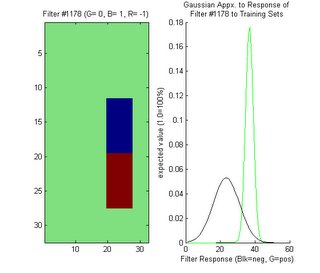
Results

Best Filter

I ran the aformentioned algorithm for all filters and for 10 positive test images. I then arranged the filter numbers according to how many votes each one had. Here is an example of one of the best filters, showing histograms of its training set with fitted gaussians (first below) and the same filter with just its gaussians displayed (second below)





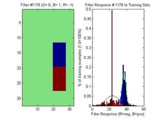
In my most recent blog posting, I displayed a filter and its response as two nested gaussians. From the experiments I have performed since then, I realize that this graph from the previous posting was obviously incorrect. When displaying the gaussians, the prior probabilities should not be taken into account. The gaussians alone are only used to compute a likelyhood estimate --not a probability. The introduction of scaling by the prior probabilities should only be added when classifying --not visualizing the PDF. I also discovered a minor bug that was causing the mean values to be shifted incorrectly. These problems have been fixed since then.
Initially, I thought that my intuition about the location of possible features did not directly translate to the use of filters in Bayes' classifiers. Now, I can see that my intuition is confirmed by the location of this filter at almost the same location as the nested gaussian in the previous post.

Worst Filter

Here is an example of one of the worst filters, displayed in the same manner as the previous two images:





Here, the gaussians almost match up meaning that the classification of an input image is almost entirely dependent on the prior probabilities. This means that if this filter were to be used to build a classifier, then training sets might as well not have been collected at all.


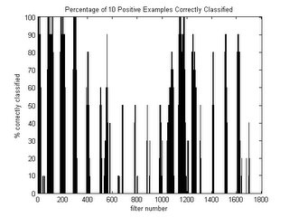
Global Analysis of Filter Performance

The graph below shows y percentage of filters that classified x percentage of test images correctly:



If you observe the far left-hand column, you can see that 80% of the filters are completely worthless in that they were not able to identify any letter 'e's correctly out of the 10 test images. One of the main advantages of Adaboost is that the presence of these useless filters will not affect the resulting strong classifier --Adaboost will automatically throw these filters out and choose the best ones. If you look at the far right-hand column, you will see that fewer than 5% of the filters classified all 10 of the test images correctly. It could be that the 10 test images I chose have attributes that make them easy to recognize by the top 5% of classifiers. Perhaps the top 5% classifiers would fail miserably with negative examples or most other positive examples. Adaboost will help to avoid this scenario by forcing the classifiers to focus on the most difficult examples.

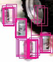
The following graph represents the percentage of test images classified correctly for each filter number. For reference, an image of the filters is shown below it:





From the graph, there are many instances where a small group of filters perform exceptionally well while a different group in close proximity performs poorly. Though only 10 examples were used to test, the advantage of generating many different filters is apparent. If intuition alone is relied upon for the construction of a filter, then it could be missing an area of interest by a few pixels that might make the difference between achieving good classifications or not. Regardless of how good human intuition is, it is handy to rely upon the precision of a computer to pick up the slack.

What's Next

The next step will be to implement Adaboost using the weak classifiers I have constructed. I may need to generate more filters, but I will keep the number small for now for the sake of computation time.

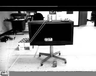
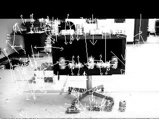
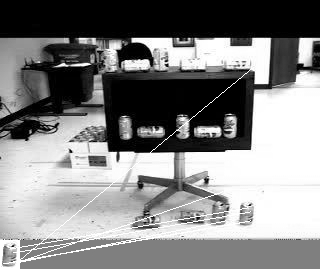
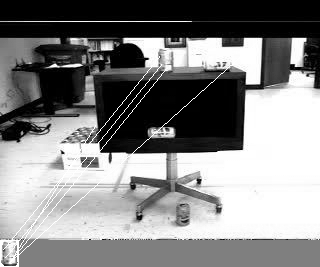
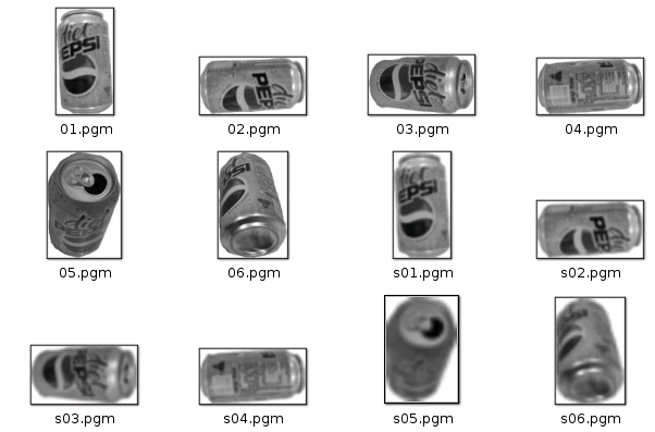
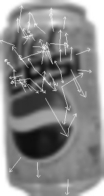
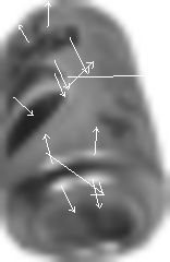
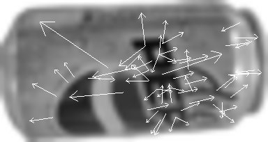
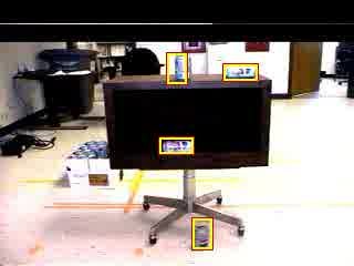
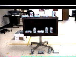
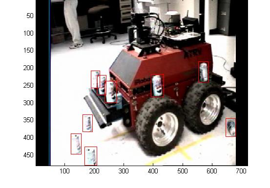
Training Footage of Soda Cans

I obtained training footage from Robart III of soda cans! I will post on this once I clean up the raw footage a bit.

Detecting the letter 'e'

Last week, I was reading over Dlagnekovs code in an attempt to understand how he used Adaboost. Dlagnekov's code is very clean and easy to understand. However, I had a difficult time discerning details from the code, such as how his Bayes classifiers work. I was also unclear as to how one is able to use a training set of images in conjunction with a group of weak classifiers to generate ROC curves. It is one thing to read theory on this subject, but I needed to see a concrete example.

I wrote up a trivial example of generating a training set and applying classifiers on paper, but I wasn't getting a nice looking graph with two distinct humps. Instead, I was getting an almost flat curve for the positive training set and two impulses for the negative training set. I talked with my professor and he said that the type of classifiers Dlagnekov uses are statistical classifiers, meaning that in order to get good curves, one must have a large number of positive and negative classifiers. He suggested that I implement an Adaboost method for detecting the letter "e" (lowercase) on a white sheet of paper before attempting to detect soda cans. He provided me with a link to a research paper that was first printed out with a dot-matrix printer, then scanned in and converted to PDF format. This means that the letters in the paper vary quite a bit, making the detection process nontrivial. He suggested that I use this paper to generate positive and negative training examples as well as using it to test my implementation. Here is a link to the paper I used:

http://www-cse.ucsd.edu/classes/sp02/cse252/foerstner/foerstner.pdf

Creating the Positive Training Set

I wanted each image to be 32x32 pixels so I zoomed in with Adobe Reader to a 400% scale and took a screenshot. I then pasted the screenshot into Windows Paintbrush and manually cut out every lowercase "e" in the image. I repeated this process until I had 100 different lowercase "e"s in a single bitmap image. This image was then run through a Matlab script I wrote where, when I click the center of each letter 'e', a 32x32 pixel region surrounding the selected location is automatically exported as a new bitmap file. I also saved the image with every lowercase "e" removed so I could later use this e-less image to create negative training examples. Since the research paper was scanned-in with a dot-matrix printer, the quality of each letter e is slightly different --some e's are almost perfect while others look more like o's. These images make up my positive training set, meaning they are examples of what the letter 'e' should look like. Here is a composite image consisting of all of the 32x32 images of the letter 'e' created for visualization purposes using a matlab script:



Creating the Negative Training Set

Using the exact same method I used to extract the letter e, I manually extracted 20 instances for each of the letters 'c','o', and 'a' since these letters appear to have features in common with the letter e, making them difficult to distinguish in some cases. I then took the images without the letter 'e' in them and ran I matlab script I wrote to automatically find and extract 400 random 32x32 areas from the e-less images. I now had my negative training set, meaning they are examples of what the letter 'e' should not look like.



Creating the Filters for the Weak Classifiers

Before I can create a group of Bayes classifiers to run through Adaboost, Each classifier needs to have a filter. Each filter does not have to be very good (in fact, if it is too good it might affect the results of Adaboost negatively) but it should yield a response that will be classified as correct for more than 50% of the time. A classifier that is correct exactly 50% of the time means that it randomly guesses if the image it is testing is a letter 'e'. One question that may arise would be "how do you know how to generate a filter that will work well with Adaboost?". The answer is basically "you don't have to". This is because Adaboost will automatically determine which filters are the best by measuring the accuracy of each weak classifier corresponding to each filter. So, in order to allow Adaboost to select effective filters, the trick is to choose "quantity" over "quality". Each filter should concentrate on a small area of the image and should be fast to compute. Initially, I generated about 7800 different filters where the sum of certain areas of the filter are subtracted from the sum of the other areas of the filter. This is done by setting some pixels to be -1 and others to be 1. When each 32x32 pixel filter is convolved with a 32x32 pixel image, this yields the same result. Dlagnekov did the same thing in his paper, but he used an optimization technique called integral images so that he would not have to compute the sum of every pixel region every time --the sum at different rectangular areas of each image is precomputed and stored. The 7800 filters that I generated didn't seem to work very well. Some of the filters I made consisted of a 2x2 pixel square moved at all possible image locations but these filters didn't seem to yield distinctive responses between the positive images and negative images. So, I looked at two research papers on generating filters using Haar-like features. This basically means that they took the difference between different regions like I did but they used larger-sized rectangles that were evenly divided into between 2 and 4 regions before their sums were subtracted. I decided to create a new Matlab script to generate a new set of filters that more closely resemble Haar-like features:



To generate this set of filters, I opened up an image of the letter 'e' in a photo-editor called Gimp and tried to identify regions of the letter 'e' that might yield a good classification. I figured that the following colored regions might be areas with good features:



The region to the right measures to be around 16x8 pixels, so I generated filters where all pixels were black except for a single 16x8 region where half of the pixels had value 1 and the other half had value -1.

Creating a Bayes Weak Classifier

In order to turn a particular filter into a Bayes classifier, there are 3 main steps that should be taken:

1) convolve the filter with all negative and positive training images and generate a separate histogram for each. Set the range of each histogram to be from the minimum value of both positive and negative responses to the maximum value of these responses. L1 Normalize each histogram by dividing the height of each bin by the sum of all of the bins. This will make the sum of each histogram add up to 1.

2) find the prior probability of finding the letter 'e' and the prior probability of finding a letter other than e. This means "if I pick a letter at random from a random piece of paper, what are the odds that the letter I pick is the letter 'e' ?". I asked my professor about this and he searched Google to come up with a probability of about 12% of finding the letter 'e'. The probability of finding a letter other than e is 100-12 = 88%.

3) find the mean and standard deviation of each set of responses, before they are binned into the histogram

When all 3 of these steps are done, the values generated are plugged into an equation that will basically fit a gaussian curve to each histogram, resulting in two humps.
The equation to use is:

(1 / ( sqrt(2*pi)*s)) * p * e^ - ( ((x-m)^2)/(2*s^2) )

where s,m is the standard deviation and mean from step 3, p is the prior probability from step 2, and x is the values of the x-axis of each histogram (ie: the values of the filter responses used to set the histogram bins).

When the two curves are generated, a cutoff point is set where anything to one side of the cutoff point is considered to be an 'e' and anything to the other side is considered to not be an 'e'. If a classifier is effective, then when the response of a new image is taken with the classifier's filter, this response should fall to the correct side of the cutoff point. If it falls to the side marked by the positive responses, then the image in question is considered to be the letter 'e' and "true" is returned. Otherwise, "false" is returned.

Generating Responses

When I graphed the response of a particular filter where a 16x8 pixel region was located on the right side, I got two curves completely inside each other. This is completely the opposite of what I thought would happen. I thought that since the right side of the letter 'e' looks different than the letters c,o, and a, then a filter with a 16x8 pixel window here would generate good responses. I wanted to make sure that at least some of my filters were good before I tried to run Adaboost on them. Otherwise, I would not know if Adaboost was working well or not. I talked with my professor and he suggested that I generate Bayes classifiers for each curve, calculate the error for each classifier, and determine which classifiers have the lowest error. The filters that perform the best will yield classifiers with the lowest calculated error. This way, I can reliably determine which curves have the lowest error rates and thus the best classification rates. This will provide a way to gauge the effectiveness of Adaboost as well as the quality of my generated filters.



Papers Reffered to

/*frequency of letter e*/
http://cm.bell-labs.com/cm/ms/what/shannonday/shannon1948.pdf

/*Haar-like features*/
http://citeseer.ist.psu.edu/viola01rapid.html
http://citeseer.ist.psu.edu/mohan01examplebased.html

/*dot-matrix scanned paper for training set*/
http://www-cse.ucsd.edu/classes/sp02/cse252/foerstner/foerstner.pdf